What is a wave?
Waves are everywhere
Waves are among the most universal physical phenomena. They appear in many different contexts throughout nature:
- Waves on the surface of water.
- Sound waves in matter, including sound in air, medical ultrasound, and seismic waves in the Earth.
- Waves on strings, such as the strings of musical instruments.
- Electromagnetic waves, including visible light, radio waves, and X-rays.
- Gravitational waves, which are ripples in space and time itself.
Waves can travel through space and carry energy and information over long distances. Everything you hear and everything you see reaches you as a wave.
A propagating dynamical disturbance
What do all of these very different phenomena have in common? A short definition that covers all of them is that a wave is a propagating dynamical disturbance. Let’s look at what each of these three words means, starting with the last one.
For now, we will focus on mechanical waves. In a mechanical wave, the “disturbance” is a displacement of the particles in a material, which we call the medium of the wave.
Disturbance: mechanical waves
For example, in a wave on the surface of a pond, the medium is the water, and the disturbance is the up-and-down displacement of the water’s surface away from its flat, undisturbed level.

Photo: Roger McLassus, “2006-01-14 Surface waves,” Wikimedia Commons, licensed under CC BY-SA 3.0.
Propagating
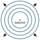
“Propagating” is another word for “traveling.” If we disturb the surface of a pond, for example by tossing a rock into the water, the disturbance travels outward from its source.
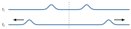
Even though the disturbance travels, the water largely stays where it is. The surface level of the water moves up and down, but the water itself doesn’t flow outward.
Dynamical
“Dynamical” means “changing over time.” As a wave propagates, the motion of the medium at each point is constantly changing. If you watch any one spot on the pond, the water there rises and falls as the ripples pass by. A moment later, a spot farther out does the same thing.
So a mechanical wave is a disturbance of a medium (like the displacement of the water’s surface) that travels from place to place (propagating) and changes with time at every point it reaches (dynamical).
Oscillations vs. waves
Many students find it difficult to distinguish oscillations and waves. There are many connections between these phenomena, but it is important to understand how they differ.
An oscillation is the motion of a single particle or object, like the mass on a spring or the bob of a pendulum. A mechanical wave is a collective motion of a huge number of particles in a medium.
Simple harmonic motion is always sinusoidal. Waves don’t have to be sinusoidal, although we will spend most of our time talking about sinusoidal waves.
Waves on a string
A model system for waves
We used the ideal gas as a model system for thermodynamics and the mass on a spring as a model system for simple harmonic motion. In the same way, we will use waves on a string as a model system for waves. Most of the physics we use to describe waves on a string also applies to other kinds of waves, like water waves, sound waves, and electromagnetic waves.
A pulse on a string
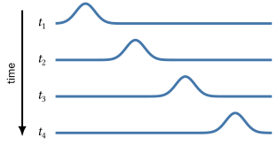
If we disturb a stretched string, by plucking it or by quickly moving one end up and down, we can create a pulse that travels along the string. The figure shows a string carrying a wave pulse at four successive times. In the idealized model we will use, the pulse keeps its shape as it moves to the right.
Is a pulse a wave?
You may think this doesn’t look like a wave, perhaps because it doesn’t look “wavy,” or because you are used to waves being sine waves.

But think about a wave as a propagating dynamical disturbance, and there should be no doubt that this is a wave! It’s a disturbance (a displacement of the string) that travels along the string, and the displacement of each point on the string changes with time as the pulse passes by.
In the rest of this chapter, we will describe waves on a string quantitatively. How fast does a wave travel, and what sets that speed? How do we write down a wave as a mathematical function?
Wave speed
The speed of a pulse
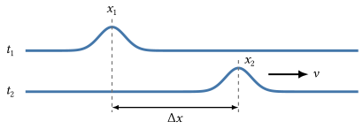
On an ideal string, a wave maintains its shape and travels at a steady speed. If its peak moves a distance $\Delta x$ in a time $\Delta t$, the wave speed is
\[v = \frac{\Delta x}{\Delta t}.\]The wave speed is the speed of the disturbance. Each piece of the string only moves up and down and does not travel with the pulse.
The medium sets the wave speed
If you send pulses of different shapes and sizes along the same string, they all travel at the same speed. The wave speed is a property of the medium, the string, not of the particular wave.
The wave speed does change if you change the string. The wave speed is higher on a string that is under greater tension, and it is lower on a string that is more dense (larger mass per unit length).
This also applies to other kinds of waves. Sound travels at the same speed through the air regardless of its pitch or loudness, but a sound wave moves through water at a different speed than in air.
Wave speed on a string
For a string with tension $F_T$, the wave speed is
\[\boxed{v = \sqrt{\frac{F_T}{\mu}}.}\]Here $\mu$ (Greek “mu”) is the linear mass density of the string, its mass per unit length. A uniform string of mass $M$ and length $L$ has
\[\mu = \frac{M}{L}.\]The SI unit of $\mu$ is $\mathrm{kg/m}$. A thick, heavy guitar string has a larger $\mu$ than a thin, light one.
Checking the units, $\sqrt{\mathrm{N}/(\mathrm{kg/m})} = \sqrt{(\mathrm{kg\,m/s^2})(\mathrm{m/kg})} = \mathrm{m/s}$.
Example: A pulse on a rope
You stretch a rope of length $4.00\ \mathrm{m}$ and mass $0.640\ \mathrm{kg}$ between two posts, with a tension of $100\ \mathrm{N}$. You flick one end to send a pulse along the rope.
- What is the linear mass density of the rope?
- What is the wave speed on the rope?
- How long does the pulse take to reach the other end?
Solution
1. The linear mass density is the mass per unit length,
\[\mu = \frac{M}{L} = \frac{0.640\ \mathrm{kg}}{4.00\ \mathrm{m}} = 0.160\ \mathrm{kg/m}.\]2. The wave speed is
\[v = \sqrt{\frac{F_T}{\mu}} = \sqrt{\frac{100\ \mathrm{N}}{0.160\ \mathrm{kg/m}}} = 25.0\ \mathrm{m/s}.\]3. The pulse travels the length of the rope at this speed, so it takes a time
\[\Delta t = \frac{L}{v} = \frac{4.00\ \mathrm{m}}{25.0\ \mathrm{m/s}} = 0.160\ \mathrm{s}.\]Wave functions
The wave function
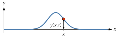
To describe a wave on a string, we’ll take our $x$-axis along the length of the string. Let $y$ be the displacement of the string from its undisturbed position, measured perpendicular to the string.
The displacement is different at different points along the string, and at each point it changes with time. This means that $y$ is a function of both position and time, $y(x,t)$, called the wave function. The wave function describes the disturbance, in that it tells us how far the medium is displaced at every position and every instant in time.
Two ways to graph a wave
The wave function depends on two variables, but an ordinary graph has only one horizontal axis. No single graph of this kind can show the full behavior of a wave, although an animation can. To graph the displacement, we have to choose to keep one of the two variables fixed:
- A snapshot is a plot of $y$ versus $x$ at fixed time $t$. It shows the shape of the whole string at one instant, like a photograph.
- A time trace is a plot of $y$ versus $t$ at fixed position $x$. (Your book calls this a “history plot.”) It is a position vs. time graph for a single point on the string, like the graphs of $x(t)$ in the chapter on simple harmonic motion.
Snapshots of a pulse
Here are five snapshots of a pulse moving to the right, taken at equal time intervals. This pulse has a steep front edge and a longer tail. The red dot marks the point on the string at the position $x_P$. Even though the wave travels horizontally, the string only moves up and down.
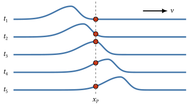
The time trace of one point
The time trace of the marked point shows its displacement at every instant. The dots show its displacements in the five snapshots.
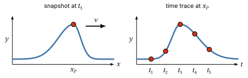
Notice that, for this pulse traveling to the right, the time trace is the mirror image of the snapshot, with the steep side first.