Macrostates, microstates, and multiplicity
What is entropy?
So far, we have explored a macroscopic view of entropy and the second law. From this perspective, the second law tells us that certain processes are impossible, but it doesn’t really tell us why they are impossible. Although we have discussed how to calculate entropy changes for certain processes, exactly what the entropy means is unclear.
This mirrors the historical development of entropy. The macroscopic formula for entropy change $\Delta S = Q/T$ was introduced by Clausius in 1854, but it took another twenty years before Boltzmann deduced what this formula actually measures. To understand the concept of entropy and the meaning of the second law more deeply, we need to investigate the connection between the macroscopic and microscopic views of a thermodynamic system.
Macrostates and microstates
The macroscopic state or macrostate of a thermodynamic system is a description of a system in terms of macroscopic properties, such as temperature, pressure, and volume. By focusing on these macroscopic properties, we are ignoring the details of the microscopic particles in the system.
In contrast, the microscopic state or microstate of a thermodynamic system is a description of the system in terms of the detailed properties of its microscopic components. For example, in a gas, the microstate is specified by the positions and velocities of all the individual particles in the system.
Speeds in a gas
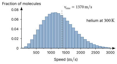
Consider the distribution of speeds in a gas, which we looked at in the chapter on kinetic theory. For this example, we can take the macrostate to be determined by the temperature of the gas, and the microstate is specified by the individual speeds of all the particles in the gas.
Heights in a population
Another example we looked at is the distribution of heights in a population of people. If we want to describe the distribution as a whole, we can give a few summary statistics of the distribution, such as the average height. These properties correspond to the macrostate of the distribution.
On the other hand, the microstate of the distribution is the complete list of the heights of all the individuals in the population. Knowing just a summary statistic like the average height tells us almost nothing about the individual heights of the people in the population. There are many different microstates that correspond to the same macrostate.
Suppose we have a population with just one person. If the average height of the population is $167\ \mathrm{cm}$, then we know for certain that the one person in the population is $167\ \mathrm{cm}$ tall. In this case, there is only one microstate that corresponds to the macrostate.
Now consider a population with two people. If the average height of the population is $167\ \mathrm{cm}$, then there are many different combinations of heights that the two people could have that would yield the same average height. Imagine playing a game where you are asked to bet on the heights of two people, given that you know their average height (and nothing else). How confidently would you be able to guess?
Multiplicity
With two people in the population, you have some hope of getting lucky and guessing the heights. As the number of people in the population increases, guessing everyone’s heights correctly quickly goes from extremely unlikely to effectively impossible.
More generally, when we describe a system using only its macroscopic properties, we are discarding a huge amount of information about the microscopic details, because there can be many different microstates that correspond to the same macrostate.
The number of microstates that correspond to a given macrostate is called the multiplicity of that macrostate, denoted $\Omega$ (capital omega):
\[\boxed{\Omega = \text{number of microstates corresponding to a given macrostate}}\]To understand the microscopic meaning of entropy, we will first need to understand what the multiplicity of a macrostate means and how to calculate it.
A toy model: coin flips
Microstates and macrostates of coin flips
To help understand multiplicity better, let’s consider a simple toy model: flipping a fair coin multiple times. Each flip of the coin can result in one of two outcomes, heads (H) or tails (T), and both outcomes are equally likely.
In this example, the microstate of the system is the specific sequence of heads and tails we get. We will take the macrostate to be specified by the total number of heads $n$ we get in the sequence. The multiplicity $\Omega(n)$ is the number of different sequences of heads and tails that yield the same total number of heads $n$.
For $N=2$ coin flips, we have the following possible microstates:
| Microstate | Macrostate ($n$) |
|---|---|
| HH | 2 |
| HT | 1 |
| TH | 1 |
| TT | 0 |
Counting the number of microstates that correspond to each macrostate, we find that the multiplicities are $\Omega(2)=1$, $\Omega(1)=2$, and $\Omega(0)=1$.
For $N=3$ coin flips, we have
| Microstate | Macrostate ($n$) |
|---|---|
| HHH | 3 |
| HHT | 2 |
| HTH | 2 |
| THH | 2 |
| HTT | 1 |
| THT | 1 |
| TTH | 1 |
| TTT | 0 |
In this case, the multiplicities are $\Omega(3)=1$, $\Omega(2)=3$, $\Omega(1)=3$, and $\Omega(0)=1$.
Example: Multiplicity of four coin flips
Extend the tables to $N = 4$ coin flips.
- List the microstates, and find the multiplicity $\Omega(n)$ of each macrostate.
- Which macrostate has the largest multiplicity? How many microstates are there in total?
Solution
1. We group the sequences by their number of heads and count each group:
| Macrostate ($n$) | Microstates | $\Omega(n)$ |
|---|---|---|
| 4 | HHHH | 1 |
| 3 | HHHT, HHTH, HTHH, THHH | 4 |
| 2 | HHTT, HTHT, HTTH, THHT, THTH, TTHH | 6 |
| 1 | HTTT, THTT, TTHT, TTTH | 4 |
| 0 | TTTT | 1 |
The multiplicities are $\Omega(4) = 1$, $\Omega(3) = 4$, $\Omega(2) = 6$, $\Omega(1) = 4$, and $\Omega(0) = 1$.
2. The macrostate $n = 2$, two heads and two tails, has the largest multiplicity, $\Omega(2) = 6$. Adding the multiplicities gives the total number of microstates:
\[\Omega_{\mathrm{tot}} = 1 + 4 + 6 + 4 + 1 = 16.\]Multiplicity for many coin flips
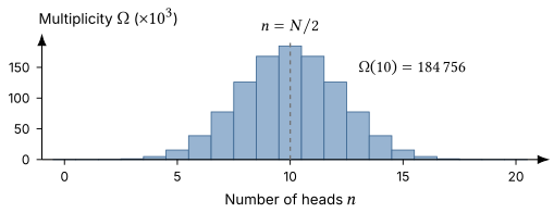
For larger numbers of coin flips, it becomes tedious to list all the microstates and count the multiplicities. However, there is a general formula for the multiplicity of a macrostate with $n$ heads in $N$ coin flips, which we will not write out here. For example, here is a plot of the multiplicity $\Omega(n)$ for $N=20$ coin flips.
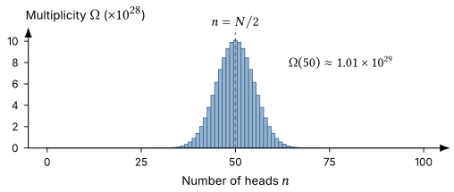
Here is the same plot for the case of $N=100$ coin flips. Notice that the multiplicity is sharply peaked around $n=N/2$. Intuitively, this should make sense: if we flip a fair coin many times, we expect to get roughly equal numbers of heads and tails.
Multiplicity and probability
Multiplicity and uncertainty
The multiplicity of a macrostate tells us how uncertain we are about the microstate of a system, given that we know its macrostate. Suppose your friend tosses a coin 3 times and tells you that they got 2 heads. If you try to guess the sequence they got, you have 3 different sequences to choose from: HHT, HTH, or THH. So just guessing randomly, you have a 1 in 3 chance of guessing correctly.
Check your understanding: Your friend tosses a coin 4 times.
- They tell you that they got 2 heads. What is your chance of guessing their sequence correctly?
- What is your chance if they tell you that they got 4 heads instead?
- Which of the two reports tells you more about the microstate? How is your answer related to the multiplicity?
Answer
1. From the previous example, $\Omega(2) = 6$ sequences have 2 heads, and each is equally likely, so a random guess is right with a chance of 1 in 6.
2. Only one sequence, HHHH, has 4 heads, so $\Omega(4) = 1$. You are certain to guess correctly, a chance of 1 in 1.
3. The report of 4 heads tells you more, because it identifies the microstate exactly. Its macrostate has the smaller multiplicity, so it leaves fewer possible microstates. The larger the multiplicity of a macrostate, the less we know about the microstate.
Multiplicity and probability
Another way to look at this is that the multiplicity tells us how likely it is that a system will be found in a given macrostate. Since each of the $2^N$ sequences of $N$ coin flips is equally likely, the probability of getting $n$ heads is proportional to the multiplicity $\Omega(n)$:
\[P(n) = \frac{\Omega(n)}{\Omega_{\mathrm{tot}}}.\]If you flip a coin 20 times, you are much more likely to get 10 heads than 0 or 20 heads, because there are many, many more sequences of coin flips with 10 heads ($\Omega(10)=184756$) than there are with 0 or 20 heads ($\Omega(0)=\Omega(20)=1$).
Equally likely microstates
For coin flips, we know that if the coin is fair and the flips are independent, then every individual sequence of heads and tails is equally likely. HHHTH is no more or less likely than HHHHH.
A physical system like a gas is much more complicated. Since a microstate has to specify the state (position and velocity) of each individual molecule, there are an enormous number of microstates, and there is no way to measure how likely each microstate is. If we want to apply the same reasoning we used for coin flips to a real system, we have to make an assumption: for an isolated system in equilibrium, all accessible microstates are equally likely.
As the molecules in a gas move around and collide with one another, over time the system will explore all of its accessible microstates at random. Combined with the assumption of equally likely microstates, this tells us that if we watch the gas for a while, the fraction of the time it spends in a given macrostate is proportional to the multiplicity of that macrostate. The macrostate we actually observe is the one with the most microstates.
Multiplicity and entropy
Entropy measures multiplicity on a logarithmic scale
When the number of particles in a system is large, the multiplicity of a macrostate can be extremely large. We saw that for a sequence of just 100 coin flips, the multiplicity of the macrostate with 50 heads and 50 tails is $\Omega = 1.01\times 10^{29}$. For a macroscopic system with $N\sim 10^{23}$ particles, the multiplicity of a macrostate can be on the order of $10^{10^{23}}$ or larger.
When dealing with extremely large numbers, it is often more convenient to measure on a logarithmic scale. In particular, we can define the entropy $S$ of a macrostate as the natural logarithm of its multiplicity:
\[\boxed{S = k_B \ln \Omega}\]The factor of $k_B$ is just a unit conversion factor to match historical thermodynamic entropy units.
Increasing entropy is overwhelmingly likely
A system is most likely to be found in the macrostate with the largest multiplicity. Since entropy is just multiplicity measured on a logarithmic scale, this means that the highest entropy macrostate is the most likely macrostate.
How much more likely? For 100 coin flips, 50 heads ($\Omega \approx 10^{29}$) is $10^{29}$ times more likely than 100 heads ($\Omega = 1$). For $N \sim 10^{23}$ particles, the ratio between the most likely macrostate and a noticeably different one is more like $10^{10^{20}}$. In equilibrium, macrostates with less than the maximum entropy are so improbable that they are never observed.
A system that starts in a low-entropy macrostate and is left alone is overwhelmingly likely to end up in the macrostate of maximum entropy, and to stay there. That macrostate is what we call thermal equilibrium.
This is the microscopic meaning of the second law. Entropy is not forbidden from decreasing. It is just so fantastically unlikely that it never happens for a macroscopic system.
Free expansion revisited
In the previous chapter, we found that a gas expanding freely from $V/2$ to $V$ increases in entropy by $\Delta S = nR\ln 2$. We can now use the microscopic definition of entropy to see where this comes from.
Before the partition is removed, all of the molecules are in one half of the container. After we remove the partition, each molecule can be in either half, so the number of positions each molecule can be in doubles. For $N$ gas molecules, the total number of arrangements increases by a factor of $2^N$:
\[\frac{\Omega_{\mathrm{f}}}{\Omega_{\mathrm{i}}} = 2^N.\]The entropy change is therefore
\[\Delta S = k_B \ln \Omega_{\mathrm{f}} - k_B \ln \Omega_{\mathrm{i}} = k_B \ln 2^N = N k_B \ln 2 = nR \ln 2,\]which is the same result we found in the previous chapter.
Although it is theoretically possible for all of the gas molecules to return to the left half of the container, this will never happen. The probability of finding all $N$ molecules there at once is $2^{-N}$, which is effectively zero for $N \sim 10^{23}$.
Two views of entropy
- Macroscopic: entropy is a state function that we measure through reversible heat flow, $\Delta S = Q_{\mathrm{rev}}/T$. The second law says $\Delta S_{\mathrm{tot}} \ge 0$.
- Microscopic: entropy counts how many microstates are consistent with what we know about a system, $S = k_B \ln \Omega$. The second law says a system evolves toward the macrostate with the most microstates, because that is overwhelmingly the most probable outcome.
Entropy and disorder
Is entropy disorder?
You may have heard entropy described as a measure of “disorder.” That description is common, but “disorder” is an informal description, and it doesn’t always align with the definition of entropy.
Instead, it is better to think of entropy as a measure of our uncertainty about a system’s microstate. As we saw with coin flips, the multiplicity tells us how uncertain we are about the microstate of a system, given that we know its macrostate. The entropy $S = k_B \ln \Omega$ measures the same uncertainty on a logarithmic scale.
In some cases, a system that looks disordered really does have more microstates than one that looks ordered, and the two ideas agree. A good example is the difference between a perfect crystal and a gas.
A perfect crystal
In a perfect crystal, every atom sits at its own site in a regular lattice. If we cool the crystal toward absolute zero, it settles into its single lowest-energy state. Then knowing the macrostate tells us the microstate: only one arrangement of the atoms is consistent with it. There is no uncertainty about the microstate, so
\[\Omega = 1 \quad\text{and}\quad S = k_B \ln 1 = 0.\]This is the third law of thermodynamics: the entropy of a perfect crystal approaches zero as $T \to 0$.
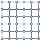
A gas
In a gas, the atoms move freely and their positions are effectively random. All the macrostate tells us about an atom is that it is somewhere inside the container.
Each atom can be anywhere in the volume $V$, so the number of places available to one atom is proportional to $V$. Counting positions alone, $N$ atoms have multiplicity
\[\Omega \propto V^N.\]This is the counting that explains free expansion. Doubling $V$ multiplies $\Omega$ by $2^N$. For $N \sim 10^{23}$, the gas has an enormous multiplicity and a large entropy.
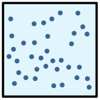
When entropy captures “disorder”
The crystal looks ordered and has $\Omega = 1$: as $T \to 0$, its entropy is $S = 0$. The gas looks disordered and has an enormous multiplicity, $\Omega \propto V^N$, and a large entropy. Here the ordered arrangement really does have lower entropy, so “disorder” is a fair description.
When “disorder” doesn’t fit
“Disorder” is an informal description of what a system looks like. A system that appears more “ordered” may in fact have more entropy than an apparently disordered system.
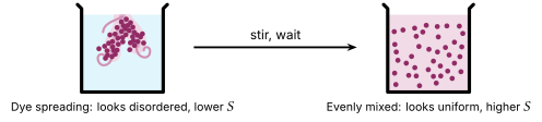
Suppose you add a few drops of soluble dye to a beaker of water. Initially, as the dye starts to spread, the beaker may appear “disordered.” If you stir the beaker and allow the system to settle, it will reach a uniform “ordered” appearance. However, a state with the dye distributed throughout the water has higher entropy than a state with the dye beginning to spread through the fluid, because there are many more microstates with the dye molecules evenly spread.