Damped oscillations
Damping and mechanical energy
In the chapters on simple harmonic motion, we ignored friction, so our model described oscillations that continued forever with the same amplitude. Real oscillating systems, if left alone, will decrease in amplitude and eventually come to rest.
Dissipative forces like friction and drag convert mechanical energy into thermal energy. By the energy principle, with no work done by external forces,
\[\Delta E_{\mathrm{mech}} + \Delta E_{\mathrm{th}} = 0.\]As thermal energy increases, the mechanical energy decreases. Since $E_{\mathrm{mech}} = \tfrac{1}{2} k_s A^2$, the amplitude of the oscillation gradually decreases. An oscillation that loses energy in this way is called a damped oscillation.
A model of damping: viscous drag
As a simple model, consider a mass moving in a viscous fluid that exerts a drag force proportional to its velocity:
\[F_{d,x} = -b v_x.\]The constant $b$ depends on the fluid and on the size and shape of the block. The minus sign means the drag force always opposes the motion. With the drag force included, Newton’s second law for the block is
\[-k_s x - b v_x = m a_x.\]The acceleration is no longer proportional to $-x$, so this is no longer simple harmonic motion. We won’t solve this equation, but we can describe what its solutions look like.
Weakly damped oscillations
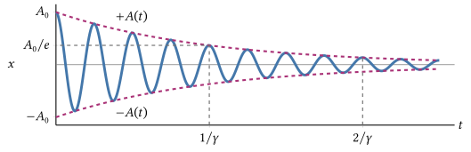
When the damping is weak, the block still oscillates, with nearly the same period as without damping. However, the amplitude decreases exponentially over time:
\[\boxed{A(t) = A_0 e^{-\gamma t}.}\]Here $A_0$ is the initial amplitude, and $\gamma = b/(2m)$ is the damping coefficient, with units of $\mathrm{s^{-1}}$.
A larger damping coefficient makes the amplitude decrease more quickly. A more viscous fluid (larger $b$) or a lighter block (smaller $m$) increases $\gamma$. With strong enough damping, the block returns slowly to equilibrium without oscillating at all. We will only consider weak damping.
The amplitude envelope
The displacement oscillates between the dashed curves $\pm A(t)$, called the envelope. Each time interval $1/\gamma$ reduces the amplitude by the same factor, $e \approx 2.72$.
Energy of a damped oscillator
With weak damping, the amplitude changes very little during one cycle, so each cycle looks almost exactly like SHM. The mechanical energy is then approximately $E_{\mathrm{mech}} \approx \tfrac{1}{2} k_s A^2$. Substituting the decreasing amplitude $A(t) = A_0 e^{-\gamma t}$ gives
\[E_{\mathrm{mech}}(t) \approx \tfrac{1}{2} k_s A_0^2 e^{-2\gamma t}.\]The energy also decreases exponentially, with $2\gamma$ in place of $\gamma$, because the energy depends on the square of the amplitude. When the amplitude has decreased to half its initial value, only a quarter of the mechanical energy remains. The mechanical energy lost by the oscillator becomes thermal energy of the block and the fluid.
Check your understanding: The amplitude of a weakly damped pendulum decreases from $10.0\ \mathrm{cm}$ to $5.0\ \mathrm{cm}$ in $20\ \mathrm{s}$.
- What fraction of its initial mechanical energy does the pendulum still have at $t = 20\ \mathrm{s}$?
- What is its amplitude at $t = 40\ \mathrm{s}$?
Answer
1. The amplitude has halved, and the mechanical energy is proportional to $A^2$, so $(1/2)^2 = 1/4$ of the initial mechanical energy remains. The other $3/4$ has become thermal energy.
2. Each $20\ \mathrm{s}$ interval multiplies the amplitude by the same factor, $1/2$. So at $t = 40\ \mathrm{s}$ the amplitude is $\tfrac{1}{2}(5.0\ \mathrm{cm}) = 2.5\ \mathrm{cm}$.
Driven oscillations and resonance
Driven oscillations
A real oscillator with a damping force eventually comes to rest. To keep it oscillating, something must add energy to replace the energy lost to damping. An external force that pushes back and forth periodically is called a driving force, and the motion it produces is a driven oscillation.
A familiar example of a driven oscillation is pushing someone on a swing. Another example is a speaker, which drives the air in front of it, producing a sound wave that in turn drives your eardrum.
We will consider a driving force that oscillates sinusoidally with driving angular frequency $\omega_d$. The oscillator also has its own natural angular frequency, the angular frequency at which it oscillates when left alone with no damping. For a mass on a spring, that is
\[\omega_0 = \sqrt{\frac{k_s}{m}}.\]Transient and steady state
When the driving force first starts, the motion is complicated. The oscillator’s own damped oscillation at its natural frequency adds to a response at the driving frequency. This early stage is the transient.
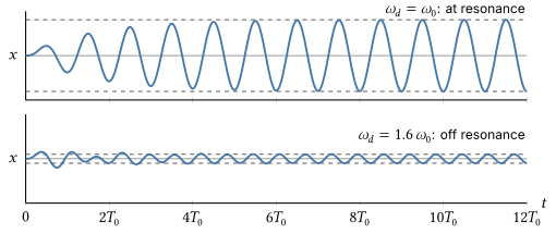
Damping makes the natural oscillation die out, just as it does for an oscillator with no driving force. The oscillator eventually reaches a steady state, in which it oscillates with a constant amplitude. In the steady state, the oscillator moves at the driving frequency $\omega_d$, not at its natural frequency $\omega_0$. Each cycle, the driving force adds exactly as much energy as damping removes.
The plots below compare two identical oscillators that start at rest at equilibrium. They are driven by sinusoidal forces with the same amplitude but different frequencies. Both graphs use the same vertical scale. The dashed lines indicate the steady-state amplitudes.
Resonance
The steady-state amplitude depends on the driving frequency and on the damping. It is largest when the driving frequency is close to the natural frequency. This large response is called resonance.
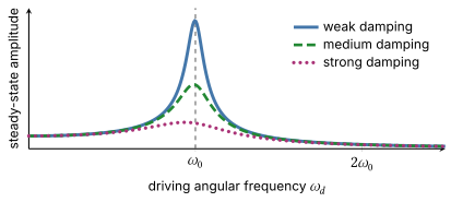
The weaker the damping, the taller and narrower the resonance peak.
Why resonance happens
Think about pushing a child on a swing. If you push once per cycle, always while the swing is moving away from you, every push adds energy. The amplitude builds up until the energy lost to damping each cycle balances the energy you add.
If you push at some other frequency, the swing ends up moving at your frequency, but your pushes no longer stay in step with its motion. For part of every cycle you push against its motion and take energy away, so the steady-state amplitude is smaller than at resonance.
Resonance happens when a driving force stays in step with an oscillator’s velocity, which requires a driving frequency close to the natural frequency. We will meet it again in musical instruments, where strings and air columns respond strongly to particular frequencies.
Example: Finding the resonance
A $0.500\ \mathrm{kg}$ block on a spring with $k_s = 200\ \mathrm{N/m}$ is weakly damped. You drive it with a sinusoidal force, slowly increasing the driving frequency from $1\ \mathrm{Hz}$ to $6\ \mathrm{Hz}$. At what driving frequency is the steady-state amplitude largest?
Solution
The natural angular frequency of the block is
\[\omega_0 = \sqrt{\frac{k_s}{m}} = \sqrt{\frac{200\ \mathrm{N/m}}{0.500\ \mathrm{kg}}} = 20.0\ \mathrm{rad/s},\]so its natural frequency is
\[f_0 = \frac{\omega_0}{2\pi} = 3.18\ \mathrm{Hz}.\]With weak damping, the resonance peak is close to the natural frequency, so the steady-state amplitude is largest for a driving frequency close to $3.18\ \mathrm{Hz}$.