Kinetic theory and molecular speeds
Kinetic theory of gases
Macroscopic properties like temperature and pressure are ultimately due to the motion of and interactions between microscopic particles. But so far, we have made no attempt to connect these two pictures.
A simple approach called kinetic theory allows us to explain the thermodynamic properties of gases from the motion of the gas molecules. In kinetic theory, we assume the molecules move at random, and that they only interact by colliding with one another, so there is no potential energy between molecules.
An analogy: heights in a population
You can think of the distribution of molecular speeds in a gas as analogous to the distribution of heights in a population of people.
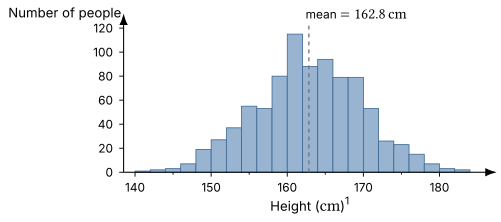
Data: CDC National Health and Nutrition Examination Survey (NHANES), public domain. Standing heights of 868 female participants aged 20–39.
The Maxwell-Boltzmann distribution
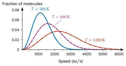
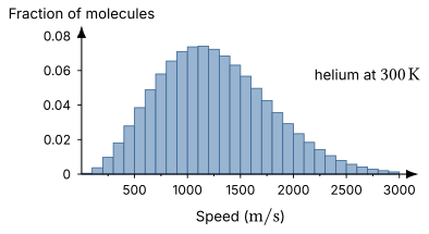
We model the distribution of speeds in an ideal gas at a given temperature $T$ by the Maxwell-Boltzmann distribution, which describes the fraction of molecules with speeds in a given interval.
Root-mean-square speed
The average kinetic energy of a single molecule is
\[K_{\mathrm{av}} = \left\langle \frac{1}{2}mv^2 \right\rangle = \frac{1}{2}m\langle v^2\rangle,\]where $\langle \cdot\rangle$ indicates the average over the speed distribution.
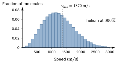
We can write the average kinetic energy in terms of the root-mean-square or rms speed, which is defined as
\[v_{\mathrm{rms}} = \sqrt{\langle v^2\rangle}.\]The name comes from the fact that we first square the speed, then take the mean, and finally take the square root. In terms of $v_{\mathrm{rms}}$,
\[K_{\mathrm{av}}=\frac12m v_{\mathrm{rms}}^2.\]For helium at $300\ \mathrm{K}$, the rms speed is about $1370\ \mathrm{m/s}$. This speed lies slightly to the right of the peak because the speed distribution has a long tail of fast molecules.
Pressure and temperature from molecular motion
Molecular motion and pressure
A gas exerts a force on its container due to collisions between the gas molecules and the walls of the container, and the gas’s pressure is related to the average speed of the gas molecules. Faster moving particles collide with the walls more frequently and with greater force, resulting in higher pressure.
We can use Newton’s second law to derive this relationship quantitatively. This derivation shows that the average force depends on the square of the velocity component perpendicular to the wall. Intuitively, increasing the velocity has two effects: stronger collisions (larger $\Delta v_x$) and more frequent collisions (smaller $\Delta t$).
Since the molecules move at random, there is no preferred direction for the velocity components:
\[\langle v_x^2\rangle=\langle v_y^2\rangle=\langle v_z^2\rangle=\frac{1}{3}\langle v^2\rangle.\]Averaging over the molecules, the average force per molecule on one wall of a container of length $L$ is
\[F_{\mathrm{av}}=\frac{m\langle v_x^2\rangle}{L}=\frac{m v_{\mathrm{rms}}^2}{3L}.\]The total force is $N$ times this average force. Dividing the force by the wall area $A$, we get the pressure in terms of the rms speed:
\[pV=\frac{1}{3}Nm v_{\mathrm{rms}}^2.\]Temperature, speed, and kinetic energy
Combining the molecular form of the ideal gas law, $pV = N k_B T$, with our pressure-speed relationship, we get
\[\frac{1}{3} N m v_{\mathrm{rms}}^2 = N k_B T.\]Rearranging, we get the rms speed in terms of the temperature and the molecular mass $m$:
\[\boxed{v_{\mathrm{rms}}=\sqrt{\frac{3k_BT}{m}}.}\]This also tells us that the average kinetic energy of a single molecule is
\[K_{\mathrm{av}}=\frac{3}{2}k_BT.\]This is an important result! It tells us that for a gas, the temperature is directly proportional to the average kinetic energy.
rms speed and temperature
Check your understanding: Compare the rms speed of a helium atom at room temperature to the rms speed of a nitrogen molecule at room temperature. The molar mass of helium is $M_{\mathrm{He}} = 4.00\ \mathrm{g/mol}$ and the molar mass of nitrogen is $M_{\mathrm{N_2}} = 28.0\ \mathrm{g/mol}$. What is the ratio of the rms speeds of the two molecules?
Answer
The rms speed of a molecule of mass $m$ in a gas at temperature $T$ is
\[v_{\mathrm{rms}} = \sqrt{\frac{3k_BT}{m}}.\]Here $m$ is the mass of one molecule, not the molar mass. One mole contains $N_A$ molecules, so $M = N_A m$, or $m = M/N_A$. Both gases are at room temperature, so $T$ is the same for both. In the ratio, the factors $3$, $k_B$, $T$, and $N_A$ all cancel:
\[\frac{v_{\mathrm{He}}}{v_{\mathrm{N_2}}} = \sqrt{\frac{M_{\mathrm{N_2}}}{M_{\mathrm{He}}}} = \sqrt{\frac{28.0\ \mathrm{g/mol}}{4.00\ \mathrm{g/mol}}} = \sqrt{7} = 2.65.\]A helium atom moves about $2.65$ times as fast as a nitrogen molecule at the same temperature. The two have the same average kinetic energy, so the lighter atom must move faster.
The speed distribution changes with temperature
The speed distribution depends on the temperature. At higher temperature, the peak in the distribution shifts to higher speed, and the distribution spreads out more.