Fluid drag forces
An object moving through a fluid (liquid or gas) experiences a force opposing its motion called fluid resistance or drag. We’ve neglected drag so far, but for real world motion, drag often plays a significant role. Just to pick a few examples, drag is essential to understand the motion of:
- a car driving on a highway
- a bacterium swimming through water
- a bird in flight
Fluid dynamics is complicated, but for many situations, we can use simple approximate models for drag forces.
Viscosity and the Reynolds number
Fluids have a form of friction called viscosity that opposes the flow of the fluid and the motion of objects through the fluid. We quantify the strength of viscosity in a fluid with the viscosity coefficient $\eta$.
Compared to water, honey flows more slowly and appears thicker because its viscosity coefficient is about 1000 times greater than that of water, even though honey has about the same density as water.
The Reynolds number $\mathrm{Re}$ is a dimensionless number that measures how much viscosity affects motion. The lower the Reynolds number, the more important viscosity is to the motion of the fluid. The Reynolds number is defined as
\[\mathrm{Re} = \frac{\rho v L}{\eta}\]where
- $\rho$ is the density of the fluid,
- $v$ is a characteristic speed (for example, the speed of an object moving through the fluid),
- $L$ is a characteristic length scale (for example, the diameter of an object moving through the fluid), and
- $\eta$ is the viscosity coefficient of the fluid.
In the limits of high and low Reynolds number, we can use simple models of the drag force:
- At high Reynolds number ($\mathrm{Re} \gtrsim 1000$) inertial drag dominates. The resistance comes from the force required to push fluid out of the way of the moving object. This is the drag force relevant for human swimmers, cars, baseballs, skydivers, etc. The drag force is proportional to the square of the speed, $F_d \propto v^2$.
- At low Reynolds number ($\mathrm{Re} \lesssim 1$) viscous drag dominates. The resistance is due to the viscous friction between the fluid and the surface of the moving object. This is the drag force relevant for microorganisms swimming through water, for example. The drag force is proportional to the speed, $F_d \propto v$.
The viscous drag force
The viscous drag force acts opposite the velocity, with a magnitude proportional to the speed:
\[\boxed{\vec{F}_{d}=-b\vec{v}}\]Here $b$ is a positive coefficient that measures the strength of the drag force. The value of $b$ depends on parameters like the shape and size of the object and the viscosity of the fluid.
For the specific case of a spherical object, the coefficient $b$ is given by Stokes’s law
\[\boxed{b=6\pi \eta r}\]where $r$ is the radius of the sphere.
Life at low Reynolds number
A famous lecture by physicist E. M. Purcell entitled Life at low Reynolds number explores the question: What is it like to be a microorganism swimming through water? Purcell explains that in the low $\mathrm{Re}$ world, the physics of motion is very different from what we are used to in our everyday lives.
For a person swimming through a pool, $\mathrm{Re}\sim 10^{5}$. However, for organisms like bacteria, $\mathrm{Re}$ is vastly smaller and viscosity dominates.
For an E. coli bacterium (diameter $L\approx 0.8\ \mathrm{\mu m}$, typical swim speed $v\approx 20\ \mathrm{\mu m/s}$) moving in water (density $\rho\approx 1000\ \mathrm{kg/m^3}$, viscosity $\eta\approx 10^{-3}\ \mathrm{Pa\,s}$), we can estimate
\[\mathrm{Re}\sim 10^{-5}.\](These values for E. coli are taken from the book E. coli in Motion by Howard Berg. If you are interested in learning more about E. coli locomotion and behavior, I highly recommend it!)
Motion with viscous drag
So, what is it like moving through a fluid at low Reynolds number, where viscous drag dominates? To answer this, let’s apply the model for the viscous drag force that we wrote down earlier:
\[\vec{F}_{d}=-b\vec{v}.\]Suppose an object starts with initial speed $v_0$ at $t=0$, and that there are no forces other than this drag force. What does the subsequent motion look like?
Taking the $x$-axis along the direction of motion, we have $F_{d,x}=-bv_x$, and Newton’s 2nd law says
\[F_{\mathrm{net},x}=-bv_{x}=ma_{x}.\]Since $a_x = \frac{dv_x}{dt}$, Newton’s 2nd law gives us a differential equation for the velocity:
\[\frac{dv_{x}}{dt}=-\frac{b}{m}v_{x}.\]Don’t worry! I’m not going to expect you to solve differential equations. But this specific equation is an important one that appears in many different contexts throughout science.
If we solve this equation to get the speed as a function of time, we find that the speed undergoes exponential decay:
\[v(t) = v_{0}e^{-\frac{b}{m}t}.\]Exponential decay
Exponential decay is a universal mathematical behavior that appears any time the rate at which a quantity decreases is proportional to the current value of the quantity.
You’ll see exponential decay again in the 5 series, and probably in several other contexts, including:
- Radioactive decay
- Charging and discharging of capacitors, which can model cell membrane potentials
- First-order chemical reaction rates
- Pharmacokinetics of drug elimination from the body
The time constant
We define the time constant $\tau$ for this motion as
\[\boxed{\tau = \frac{m}{b}}\]In terms of the time constant, we can write the speed as
\[\boxed{v(t) = v_{0}e^{-t/\tau}}\]The time constant is the characteristic time scale for exponential decay. The larger the time constant, the more slowly the speed decreases. Specifically, after a time of one time constant, the speed has decreased to $e^{-1}\approx 37\%$ of its initial value:
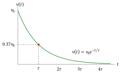
Stopping distance
In this exponential decay model, the speed of the object never actually reaches zero, but it gets arbitrarily close to zero as time goes on.
We will refer to the maximum distance the object could travel as it comes to rest as the stopping distance $\Delta x_{\mathrm{stop}}$. We can calculate this by integrating the speed over time:
\[\Delta x_{\mathrm{stop}} = \int_0^\infty v(t)\, dt.\]Evaluating this integral with the expression for $v(t)$ gives us
\[\boxed{\Delta x_{\mathrm{stop}} = v_0 \tau}\]For an E. coli bacterium swimming through water, the initial speed is on the order of $v_0 \sim 10^{-5}\ \mathrm{m/s}$, and the time constant is on the order of $\tau \sim 10^{-7}\ \mathrm{s}$, so the stopping distance is on the order of
\[\Delta x_{\mathrm{stop}} \sim 10^{-12}\ \mathrm{m}.\]This distance is much smaller than the size of a bacterium itself, even smaller than the diameter of an atom. If an E. coli bacterium stops swimming, it comes to rest essentially immediately and doesn’t coast at all.
This is one way in which motion at low Reynolds number is very different from motion at high Reynolds number. Another difference is that swimming by pushing fluid backward doesn’t work at low Reynolds number, so microorganisms have to use more complicated strategies to propel themselves through the fluid. For example, E. coli bacteria have long helical flagella that they rotate to swim forward.
Example: Half-speed time with viscous drag
A small spherical object with mass $2.0\ \mathrm{ng}$ moves through a viscous fluid. The drag coefficient for this motion is $b = 4.0 \times 10^{-5}\ \mathrm{kg/s}$. How long does it take this object to slow to half of its initial speed?
Solution
For motion with linear viscous drag, the speed decays exponentially:
\[v(t) = v_0 e^{-t/\tau},\]where the time constant is
\[\tau = \frac{m}{b}.\]We want the time $t_{1/2}$ (the “half-life”) when $v(t_{1/2}) = v_0/2$, so
\[\begin{aligned} \frac{v_0}{2} &= v_0 e^{-t_{1/2}/\tau}\\ \frac{1}{2} &= e^{-t_{1/2}/\tau}. \end{aligned}\]Taking the natural logarithm of both sides,
\[\begin{aligned} \ln\!\left(\frac{1}{2}\right) &= -\frac{t_{1/2}}{\tau}\\ t_{1/2} &= \tau \ln 2. \end{aligned}\]Now calculate the time constant. Since
\[2.0\ \mathrm{ng} = 2.0 \times 10^{-12}\ \mathrm{kg},\]we have
\[\begin{aligned} \tau &= \frac{2.0 \times 10^{-12}\ \mathrm{kg}}{4.0 \times 10^{-5}\ \mathrm{kg/s}}\\ &= 5.0 \times 10^{-8}\ \mathrm{s}. \end{aligned}\]Therefore
\[\begin{aligned} t_{1/2} &= \left(5.0 \times 10^{-8}\ \mathrm{s}\right)\ln 2\\ &= \boxed{3.5 \times 10^{-8}\ \mathrm{s}.} \end{aligned}\]