Springs and elasticity

Elastic forces and Hooke’s law

The tension in a string is one example of an elastic force: a force that is exerted by an object that undergoes a change in shape or deformation—stretching, compressing, bending, etc. In the case of a string, the change in shape is the stretching of the string, and the tension resists the stretching.

For small deformations, we can often model elastic forces as being proportional to the amount of deformation. We call this relationship Hooke’s law. A force that obeys Hooke’s law and acts to restore an object to its original shape is called a linear restoring force.

The spring force

Let’s start by looking at Hooke’s law applied to an ideal spring. A spring has a natural or unstressed length $L_0$ that it takes when no forces are applied to it.

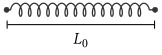
A horizontal spring at its natural relaxed length, with small dots marking each end. A measurement bracket below the spring labels its length L sub 0.

If we stretch the spring to a greater length $L$, then the spring exerts a restoring force $\vec{F}_{\mathrm{sp}}$ that points inward along the spring, trying to return to its unstressed length.

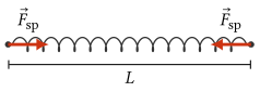
Two horizontal springs stacked vertically for length comparison. The top spring is at its natural length L sub 0. The bottom spring is stretched to a longer length L, with red restoring force vectors at each end pointing inward toward the spring's center. Length brackets below each spring label their lengths.

Similarly, if we compress the spring, the spring exerts a restoring force outward.

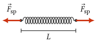
Two horizontal springs stacked vertically for length comparison. The top spring is at its natural length L sub 0. The bottom spring is compressed to a shorter length L, with red restoring force vectors at each end pointing outward, away from the spring's center. Length brackets below each spring label their lengths.

I will call the difference between the current length $L$ and the unstressed length $L_0$ the extension $s$ of the spring:

\[\boxed{s = L - L_0}\]

You can think of $s$ as standing for “stretch.” Note that $s$ is positive for a stretched spring and negative for a compressed spring.

Hooke’s law says that the magnitude of the spring force is proportional to the extension $s$:

\[\boxed{F_\mathrm{sp} = k \lvert s\rvert}\]

The reason we take the absolute value of $s$ is that $s$ can be positive or negative, but the magnitude of the spring force must be positive.

The constant $k$ is called the spring constant or force constant of the spring. It measures how stiff the spring is: a larger $k$ means a spring that is harder to stretch or compress. The units of the spring constant are $\mathrm{N/m}$.

We determine the direction of the spring force based on whether the spring is stretched or compressed:

If the spring is stretched ($s > 0$), the spring force points inward, toward the center of the spring.
If the spring is compressed ($s < 0$), the spring force points outward, away from the center of the spring.

Example: Hanging mass on a vertical spring

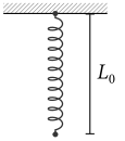
A light spring with spring constant $300\ \mathrm{N/m}$ and length $10\ \mathrm{cm}$ is suspended vertically. A $750\ \mathrm{g}$ mass is attached to the spring and slowly lowered until it comes to rest at equilibrium. What length does the spring have with the mass suspended?

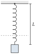
A massless vertical spring suspended from a horizontal hatched ceiling at its natural length L sub 0. A length bracket to the right of the spring labels its length.

A vertical spring hanging from a horizontal hatched ceiling, stretched downward by a block attached at its lower end. A horizontal dashed line at the unstressed length L sub 0 marks where the bottom of the relaxed spring would be. Length brackets on the left and right label the natural length L sub 0 and the stretched length L.

Solution

Let $L_0 = 10\ \mathrm{cm} = 0.100\ \mathrm{m}$ be the unstressed length, and let $s = L - L_0$ be the spring’s extension. Since the mass is at rest in equilibrium, the upward spring force balances the downward weight:

\[\begin{aligned} F_{\mathrm{net},y} &= m a_y\\ F_{\mathrm{sp}} - mg &= 0\\ ks &= mg. \end{aligned}\]

Solving for the extension,

\[\begin{aligned} s &= \frac{mg}{k}\\ &= \frac{(0.750\ \mathrm{kg})(9.8\ \mathrm{m/s^2})}{300\ \mathrm{N/m}}\\ &= 0.0245\ \mathrm{m} = 2.45\ \mathrm{cm}. \end{aligned}\]

The total length is therefore

\[\begin{aligned} L &= L_0 + s\\ &= 10.0\ \mathrm{cm} + 2.45\ \mathrm{cm}\\ &= \boxed{12.5\ \mathrm{cm}.} \end{aligned}\]

Elastic solids

A simple model for solid materials is a network of masses connected by microscopic springs. The masses represent atoms, and the springs represent the electromagnetic forces associated with the chemical bonds between atoms.

For example, we could model a string as a long chain of atoms:

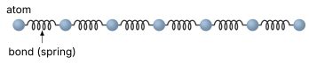
A horizontal linear chain of seven blue circles representing atoms, connected by short coil springs representing interatomic bonds. The chain represents the microscopic structure of an elastic string.

We can then treat the string as having an effective spring constant $k$ that depends on the strength of the bonds and the number of bonds in the chain.

Derivation: Springs in series

When we connect two springs end-to-end (or “in series”), the combined spring is easier to stretch than either individual spring. We can see why with a short calculation.

Connect two identical springs, each with spring constant $k$, end to end, and stretch the combination with a force $F$. Both springs must exert the same force $F$ for the system to be in equilibrium, so they both stretch by $s = F/k$. The total extension is

\[s_\mathrm{total} = s_1 + s_2 = \frac{2F}{k}\]

The effective spring constant of the combined spring is therefore

\[\boxed{k_\mathrm{eff} = \frac{F}{s_\mathrm{total}} = \frac{k}{2}}\]

That is, two springs in series act like a single spring with half the spring constant.

Derivation: Springs in parallel

Rather than a single long chain, a slightly better model for an elastic string is a collection of long parallel chains of atoms connected by springs:

Three horizontal parallel linear chains of seven blue circles representing atoms, connected by short coil springs representing interatomic bonds. The chains represent the microscopic structure of an elastic string.

Springs in parallel have a larger effective spring constant than the individual springs. Another calculation like the one for springs in series shows why springs in parallel are stiffer.

Connect two identical springs with spring constant $k$ side by side (or “in parallel”), and stretch the combination with a force $F$. Both springs stretch by the same amount $s$, and their net force must balance the applied force:

\[F = k s + k s = 2 k s\]

The effective spring constant of the combined spring is therefore

\[\boxed{k_\mathrm{eff} = \frac{F}{s} = 2k}\]

That is, two springs in parallel act like a single spring with twice the spring constant.

Cross-sectional area

The cross-sectional area $A$ is the area of a slice cut perpendicular to the length of the object. For a string, rod, tendon, etc., this means the area of the end face that would be exposed by cutting straight across the object.

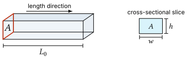
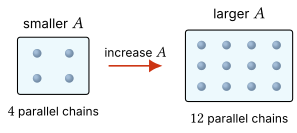
A long rectangular solid with its left end face shaded blue and outlined in red. The shaded end face is labeled cross-sectional area A. A length bracket underneath is labeled L sub 0. To the right, a rectangular cross-sectional slice is shown.

In the microscopic model, each chain runs along the length of the material. Looking at the cross section, each chain appears as one atom-sized “spot.” A larger cross section contains more chains in parallel.

Two cross-sectional slices are shown. The smaller slice contains four blue dots, each representing one spring chain running along the length. The larger slice contains twelve blue dots. An arrow from the smaller slice to the larger slice is labeled increase A, showing that larger cross-sectional area means more parallel chains.

Scaling of the spring constant of a solid

From these two derivations, we can conclude the following regarding the effective spring constant $k$ of a solid material, modeled as parallel chains of springs:

$k$ is inversely proportional to the length $L_0$ of the material, since longer chains of springs in series have a smaller effective spring constant.
$k$ is proportional to the cross-sectional area $A$ of the material, since a larger cross section contains more parallel chains of springs.

Putting these geometry effects together, the spring constant of a solid sample scales like

\[k \propto \frac{A}{L_0}.\]

Young’s modulus and stress–strain

If we introduce a proportionality constant $Y$ to turn the proportionality into an equation, we get

\[\boxed{k = Y \frac{A}{L_0}}\]

$Y$ is called the Young’s modulus of the material. It measures how stiff the material is, independent of its geometry.

The units of the Young’s modulus are $\mathrm{N/m^2}$. This combination of units is called a pascal ($\mathrm{Pa}$):

\[\mathrm{Pa} = \frac{\mathrm{N}}{\mathrm{m^2}}.\]

Stress and strain

Writing the spring constant in terms of the Young’s modulus, we can express Hooke’s law for a solid material as

\[F = k s = \left(\frac{YA}{L_0}\right) s\]

and we can rearrange this equation to get

\[\frac{F}{A} = Y \left(\frac{s}{L_0}\right).\]

The left-hand side of this equation is the force per unit area or stress on the material:

\[\boxed{\sigma = \frac{F}{A}}\]

The right-hand side is the Young’s modulus times the fractional extension of the material, which is called the tensile strain:

\[\boxed{\varepsilon = \frac{s}{L_0}}\]

In terms of the stress and strain, we can rewrite Hooke’s law for a solid material as

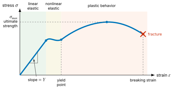
\[\boxed{\sigma = Y \varepsilon.}\]

This shows that we can interpret the Young’s modulus as the ratio of stress to strain for a material, at least for small strains where Hooke’s law applies.

Beyond Hooke’s law

The linear stress-strain relationship described by Hooke’s law is only an approximation that applies for small strains. For larger strains, the relationship between stress and strain becomes nonlinear, and the material may eventually break.

So far, we have only considered the case of elastic deformation, where the material returns to its original shape after the force is removed. If the material is stretched beyond its elastic limit, it undergoes plastic deformation, where it does not return to its original shape.

The point at which a material transitions from elastic to plastic deformation is called the yield point. If we continue to strain the material beyond the yield point, it will eventually reach its breaking point, where it fractures or breaks apart.

The maximum stress that a material can withstand before breaking is called the ultimate strength $\sigma_{\max}$ of the material. For tensile stress specifically, the ultimate strength is called the tensile strength.

$Schematic stress-strain graph. Stress is on the vertical axis and strain is on the horizontal axis. The curve begins as a straight linear elastic region whose slope is labeled Young's modulus Y, then bends into a nonlinear elastic region, crosses a yield point into plastic behavior, rises to an ultimate strength peak, then falls and ends at a fracture point. A dashed horizontal line marks the ultimate strength and a dashed vertical line marks the breaking strain.$

Example: Achilles tendon stress and strain

The Achilles tendon connects the calf muscles to the heel bone and transmits large tensile forces during walking, running, and jumping. Model the Achilles tendon as a uniform elastic cable with unstressed length $12.0\ \mathrm{cm}$ and cross-sectional area $70.0\ \mathrm{mm^2}$. The Young’s modulus of the tendon is $1.2\ \mathrm{GPa}$, and its tensile strength is $80\ \mathrm{MPa}$. During a strong push-off, the tension in the tendon is $1200\ \mathrm{N}$.

Assuming the tendon obeys Hooke’s law in this range, calculate the extension $s$ of the tendon in millimeters.
What is the maximum tension this tendon could withstand before rupturing according to this simplified model?
By what factor is the maximum tension larger than the actual tension?

Solution

First convert the geometry to base SI units:

\[L_0 = 0.120\ \mathrm{m}, \qquad A = 70.0\ \mathrm{mm^2} = 7.00 \times 10^{-5}\ \mathrm{m^2}.\]

Note that when squaring a unit with a prefix, the prefix is also squared:

\[(1\ \mathrm{mm})^2 = (10^{-3}\ \mathrm{m})^2 = 10^{-6}\ \mathrm{m^2}.\]

(a) For a solid material obeying Hooke’s law,

\[\frac{F}{A} = Y\frac{s}{L_0}.\]

Solving for $s$,

\[\begin{aligned} s &= \frac{F L_0}{Y A}\\ &= \frac{(1200\ \mathrm{N})(0.120\ \mathrm{m})}{(1.2 \times 10^{9}\ \mathrm{Pa})(7.00 \times 10^{-5}\ \mathrm{m^2})}\\ &= 1.71 \times 10^{-3}\ \mathrm{m} = \boxed{1.7\ \mathrm{mm}.} \end{aligned}\]

(b) The tendon ruptures in this simplified model when the stress reaches the tensile strength:

\[\begin{aligned} \sigma_{\max} &= \frac{F_{\max}}{A}\\ F_{\max} &= \sigma_{\max} A\\ &= (80 \times 10^{6}\ \mathrm{Pa})(7.00 \times 10^{-5}\ \mathrm{m^2})\\ &= \boxed{5600\ \mathrm{N}.} \end{aligned}\]

(c) The factor is

\[\begin{aligned} \frac{F_{\max}}{F} &= \frac{5600\ \mathrm{N}}{1200\ \mathrm{N}}\\ &= \boxed{4.7}. \end{aligned}\]