Mechanics: the physics of motion
In this class we cover mechanics, the physics of motion. Why start here? There are a few good arguments:
- You already have a lot of direct experience with motion, so it’s relatively easy to connect the concepts to your everyday experience.
- Many phenomena throughout physics can be understood in terms of motion of microscopic particles: fluid flow, diffusion, heat conduction, cell membrane potentials, sound waves, and more. Studying motion gives us a foundation for understanding these phenomena.
We can think about this course as being split up into roughly three parts:
- Kinematics: How do we represent motion? How do we make mathematical models of motion that we can use to make predictions?
- Interactions (force and torque): How do objects interact? What causes or changes motion?
- Energy: How does conservation of energy constrain motion? How can we explain motion using transfers or transformations of energy?
Measurement and coordinates
To measure motion, we need to be able to measure distance and time. To do this, we need to choose a coordinate system: a set of clocks and rulers.
We’re free to choose whatever coordinate system we want. The physics we observe will be the same in any coordinate system, but we might measure different numbers depending on the coordinates we use. Among the choices we get to make about our coordinate system:
- How are our axes oriented in space?
- Which direction along a given axis is positive?
- Where is the origin (zero point) of our axes?
- What time do we set as $t = 0$?
Units
It’s helpful to use a standard system of units to measure distance, time and other quantities. This means we decide on standard scales for our measuring devices so we can compare measurements with other people.
The most common system of units in physics, and the one we will use, is the International System of Units, or SI (from the French Système international d’unités). The SI unit of time is the second ($\mathrm{s}$), and the SI unit of length is the meter ($\mathrm{m}$). (One meter is about 3.3 feet.)
Scientific notation and unit prefixes
Values that are very large or very small in a given unit can be expressed more compactly using scientific notation, where we write a number as a product of a number and a power of 10. For example, the average distance from the Earth to the Sun is about $149{,}600{,}000{,}000\ \mathrm{m}$, which can be written as $1.496 \times 10^{11}\ \mathrm{m}$.
Instead of writing out the power of 10, we can use a unit prefix to give the same information. For example, the diameter of an E. coli bacterium is roughly $1 \times 10^{-6}\ \mathrm{m}$. Using the SI prefix micro (symbol μ), we can write this as $1\ \mathrm{\mu m}$.
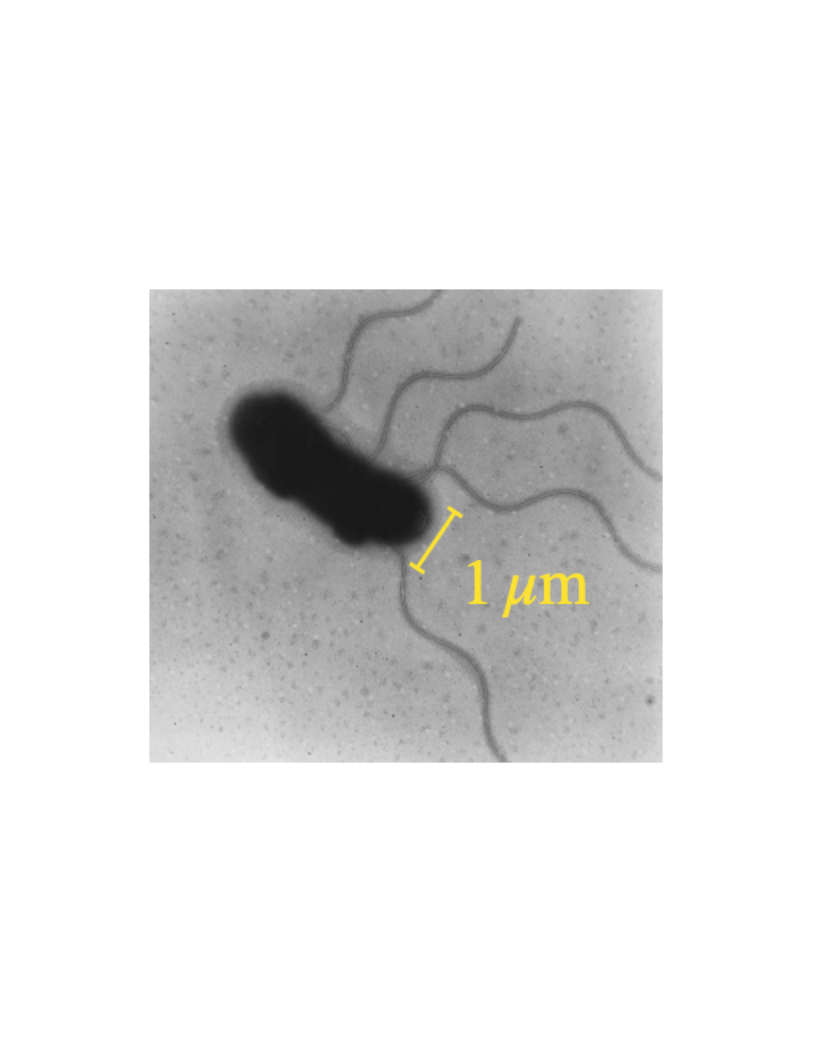
You should memorize and know how to use the following unit prefixes. These are listed in the Memorization Guide on Bruin Learn, along with the other material that you are expected to memorize for the exams.
| Prefix | Symbol | Power |
|---|---|---|
| giga | G | $10^9$ |
| mega | M | $10^6$ |
| kilo | k | $10^3$ |
| centi | c | $10^{-2}$ |
| milli | m | $10^{-3}$ |
| micro | μ | $10^{-6}$ |
The point particle model
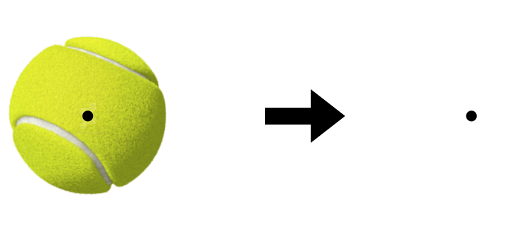
The simplest way to represent an object’s motion is with the point particle model, where we treat the object as being located at a single point in space. This allows us to represent the position of the object with a single set of coordinates.
Motion diagrams
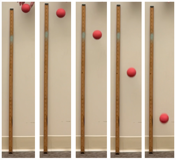
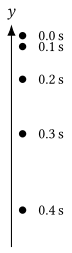
One way to represent motion is with a motion diagram, which is a simplified picture of a particle’s motion that shows “snapshots” of the particle at equally spaced instants in time. Here is a sequence of video frames of a falling ball, and the corresponding motion diagram:
Position and coordinates
To specify where a particle is (its position) at different times, we can give its coordinates at those times. The coordinates are the numbers we get when we measure the particle’s position using our chosen coordinate axes.
For example, the $y$-coordinate measurements for the falling ball taken every $0.10\ \mathrm{s}$ would look like this:
| $t$ ($\mathrm{s}$) | $y$ ($\mathrm{cm}$) |
|---|---|
| $0.00$ | $100$ |
| $0.10$ | $95$ |
| $0.20$ | $80$ |
| $0.30$ | $56$ |
| $0.40$ | $22$ |
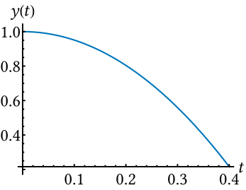
Each coordinate is a function of time. If we input a certain time $t$ into the coordinate function $y$, we get the coordinate at that time, $y(t)$. For example, $y(0.20\ \mathrm{s}) = 80\ \mathrm{cm}$ for this motion.
Position vs. time graphs
If we graph the coordinates of a particle as a function of time, we get a position vs. time graph. (In general, an “A vs. B” graph shows how one quantity A changes with respect to another quantity B. That is, the vertical axis represents A and the horizontal axis represents B.) For example, here is the position vs. time graph for a falling ball using data from a video of a ball falling from a height of $1\ \mathrm{m}$:
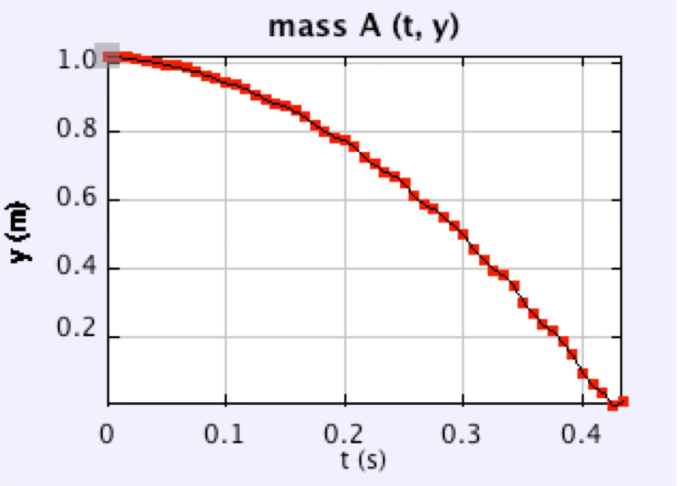
Although we can only make measurements at discrete times, we consider an idealized model of motion where our coordinates are continuous functions of time. If we plot one of these idealized coordinate functions, we get a smooth curve instead of discrete points. Here is the continuous position vs. time graph for a falling ball:
Displacement
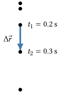
The change in a particle’s position over a time interval is called the displacement of the particle during that time interval. We use the notation $\Delta \vec{r}$ for the displacement.
One way to represent the displacement is by drawing an arrow from the particle’s initial position to its final position.
Vectors and scalars
A quantity that has both a magnitude and a direction is called a vector. Displacement is one example of a vector quantity.
- The magnitude is the numerical “amount” of the vector. For the displacement vector, the magnitude is the distance from the initial point to the final point.
- We can represent vectors graphically as arrows. The length of the arrow corresponds to the magnitude of the vector, and the direction of the arrow corresponds to the direction of the vector.
- To indicate that a quantity is a vector, we write it with an arrow above it, like this: $\vec{A}$. (The little arrow symbol above the letter always points right. Its direction is unrelated to the direction of the vector.)
- Examples of vector quantities include displacement $\Delta \vec{r}$, velocity $\vec{v}$, acceleration $\vec{a}$, and force $\vec{F}$.
- A quantity that is an ordinary number without a direction is called a scalar. Examples of scalar quantities include time $t$, distance $d$, speed $v$, mass $m$, and energy $E$.
Vector magnitude
The magnitude of a vector is always a non-negative scalar. To indicate the magnitude of a vector, we write the vector with vertical bars around it, like this: $\lvert \vec{A}\rvert $. It is also common to write the magnitude of a vector $\vec{A}$ using the same symbol without the arrow, like this: $A$. For example, if $\vec{v}$ is a velocity vector, then $v$ is the speed, which is the magnitude of the velocity.
Vector components
We can represent a vector numerically by giving its components along the coordinate axes. The components of a vector tell us the length and direction of a vector along each coordinate axis.
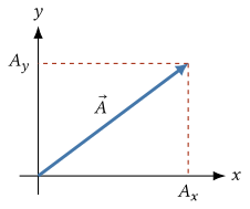
The components of a vector are the projections of the vector onto the axes. If we shine a light onto the vector perpendicular to the axes, the point where the tip of the shadow hits each axis is the component of the vector along that axis.
If a particle moves from position $\mathrm{a}$ with coordinates $(x_{\mathrm{a}}, y_{\mathrm{a}})$ to position $\mathrm{b}$ with coordinates $(x_{\mathrm{b}}, y_{\mathrm{b}})$, then the components of the displacement vector $\Delta \vec{r}$ are given by
\[\begin{aligned} \Delta x &= x_{\mathrm{b}} - x_{\mathrm{a}} \\ \Delta y &= y_{\mathrm{b}} - y_{\mathrm{a}} \end{aligned}\]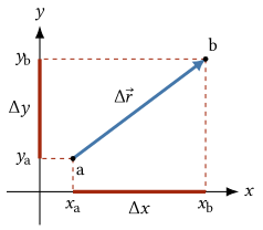
The sign of a component
The sign of a vector component (positive or negative) tells us whether the vector points in the positive or negative direction along the corresponding axis.
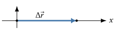
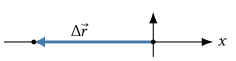
Don’t make the mistake of thinking that positive always means “to the right” or “up” and negative always means “to the left” or “down”. The sign of the components only specifies the direction relative to the direction of the coordinate axes.
A vector is defined by magnitude and direction
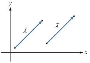
A vector is completely defined by its magnitude and direction, or equivalently by its components in a given coordinate system. This means that it doesn’t matter where the vector is located in space. Two vectors with the same magnitude and direction are the same vector, even if they are drawn in different places.
Writing vectors
We can specify a vector by listing its components in a chosen coordinate system. For example, the vector $\vec{A}$ with components $A_x$ and $A_y$ can be written as
\[\vec{A} = (A_x, A_y).\]I’ll refer to this as the component form of the vector, and it is the most common way we will write vectors in this class.
Another way to specify a vector is to give its magnitude and direction. The magnitude is a single number, and the direction can be specified in a variety of ways. For example: “up,” “Northeast,” and “$30^\circ$ above the horizontal” are all ways to specify a direction.
If a vector is parallel to one of the coordinate axes (that is, it only has one nonzero component), then the magnitude of the vector is just the absolute value of that component. For example, if
\[\vec{A} = (-3.0\ \mathrm{m},\ 0),\]then $\lvert \vec{A}\rvert = 3.0\ \mathrm{m}$.
If a vector has two nonzero components, then we can use the Pythagorean theorem to find the magnitude by treating the vector as the hypotenuse of a right triangle:
\[|\vec{A}| = \sqrt{A_x^2 + A_y^2}.\]We will see how to do this in more detail in the next chapter.
Check your understanding: In the falling ball example from earlier, the ball falls straight down. At time $t_1 = 0.20\ \mathrm{s}$, the ball is at $y_1 = 80\ \mathrm{cm}$, and at time $t_2 = 0.30\ \mathrm{s}$, the ball is at $y_2 = 56\ \mathrm{cm}$. What are the components of the displacement vector over this time interval? What are the magnitude and direction of the displacement vector?
Answer
The displacement vector is $\Delta \vec{r} = (0,\ y_2 - y_1) = (0,\ -24\ \mathrm{cm})$ or $(0,\ -0.24\ \mathrm{m})$. The magnitude of the displacement is $\lvert \Delta \vec{r}\rvert = 24\ \mathrm{cm}$, and the direction is down.