Average velocity and scalar multiplication
To describe motion, we need two pieces of information: how fast the particle is moving and in which direction it is moving. The velocity vector $\vec{v}$ tells us both of these pieces of information. The magnitude $v$ of the velocity vector is called the speed of the particle. The direction of the velocity vector is the direction in which the particle is moving.
Important: Pay attention to the difference between the velocity $\vec{v}$, which is a vector with both a magnitude and a direction, and the speed $v$, which is a scalar. The speed answers the question “How fast is the particle moving?” The velocity answers the question “How fast is the particle moving, and in which direction?”
The velocity at a particular instant in time is called the instantaneous velocity, and we will see how to define it in the next chapter. For now, we will focus on the average velocity $\vec{v}_{\mathrm{av}}$ over a time interval. Over a time interval $\Delta t = t_2 - t_1$, if a particle undergoes displacement $\Delta \vec{r}$, its average velocity vector is
\[\boxed{\vec{v}_{\mathrm{av}} = \frac{\Delta \vec{r}}{\Delta t}.}\]When we divide the vector $\Delta \vec{r}$ by the scalar $\Delta t$, we get a new vector $\vec{v}_{\mathrm{av}}$ that points in the same direction as $\Delta \vec{r}$.
Scalar multiplication
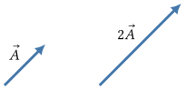
Multiplying a vector by a number scales the vector, stretching or shrinking it (hence the word “scalar”). For example, the vector $2\vec{A}$ points in the same direction as $\vec{A}$ but has twice the magnitude.
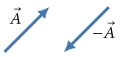
If we multiply by a negative number, we get a vector that points in the opposite direction.
In terms of the components of a vector, multiplying the vector by a scalar $c$ means multiplying each component by $c$:
\[c\vec{A} = \left( cA_x, cA_y \right).\]This means that for our average velocity, we have
\[\begin{aligned} \vec{v}_{\mathrm{av}} &= \frac{\Delta \vec{r}}{\Delta t} \\ &= \frac{1}{\Delta t} (\Delta x, \Delta y) \\ &= \left( \frac{\Delta x}{\Delta t}, \frac{\Delta y}{\Delta t} \right). \end{aligned}\]Units of velocity
Since we calculate $\vec{v}_{\mathrm{av}}$ by dividing $\Delta \vec{r}$ (unit $\mathrm{m}$) by $\Delta t$ (unit $\mathrm{s}$), the units of $\vec{v}_{\mathrm{av}}$ are $\mathrm{m/s}$, pronounced “meters per second.”
$1.0\ \mathrm{m/s}$ is about $2.2\ \mathrm{mph}$, which is approximately the speed of a person walking. Some other numbers for reference:
- A car on the freeway (without traffic) might be going $30\ \mathrm{m/s}$ ($67\ \mathrm{mph}$).
- Usain Bolt’s top speed during his world record 100 m sprint was about $12.4\ \mathrm{m/s}$ ($28\ \mathrm{mph}$).
- The Artemis II rocket orbited the Earth at a speed of about $7.8\ \mathrm{km/s}$ ($17{,}500\ \mathrm{mph}$) before heading to the Moon.
Velocity of a falling ball
Consider the example of the falling ball from the previous chapter. We had the following data for the $y$ coordinate of the ball at different times:
| $t$ ($\mathrm{s}$) | $y$ ($\mathrm{cm}$) |
|---|---|
| $0.00$ | $100$ |
| $0.10$ | $95$ |
| $0.20$ | $80$ |
| $0.30$ | $56$ |
| $0.40$ | $22$ |
Calculating the $y$-component of the average velocity between $t = 0\ \mathrm{s}$ and $t = 0.10\ \mathrm{s}$, we get
\[v_{\mathrm{av},y} = \frac{\Delta y}{\Delta t} = \frac{0.95\ \mathrm{m} - 1.0\ \mathrm{m}}{0.10\ \mathrm{s} - 0.00\ \mathrm{s}} = -0.50\ \mathrm{m/s}.\]Repeating the same calculation for the other time intervals in the table, we get the following values for the $y$-component of the average velocity:
| Time interval | $v_{\mathrm{av},y}$ ($\mathrm{m/s}$) |
|---|---|
| $0.00\ \mathrm{s}$ to $0.10\ \mathrm{s}$ | $-0.50$ |
| $0.10\ \mathrm{s}$ to $0.20\ \mathrm{s}$ | $-1.5$ |
| $0.20\ \mathrm{s}$ to $0.30\ \mathrm{s}$ | $-2.4$ |
| $0.30\ \mathrm{s}$ to $0.40\ \mathrm{s}$ | $-3.4$ |
Notice that the average velocity is changing over time. In particular, its magnitude is increasing. Measuring how motion changes over time is just as important as measuring motion itself, and this is what we will talk about next.
Average acceleration and vector addition
Let’s think about how to describe the change in velocity over time. Since velocity is a vector, we need to use vector math to describe how it changes. Suppose that over a time interval $\Delta t$, the velocity vector of a particle changes from $\vec{v}_1$ to $\vec{v}_2$.
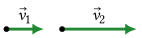
Since the velocity is a vector, the change in the velocity $\Delta \vec{v}$ over this time interval is also a vector given by
\[\Delta \vec{v} = \vec{v}_2 - \vec{v}_1.\]Another way to think about this is that $\Delta \vec{v}$ is the vector that we need to add to $\vec{v}_1$ to “update” it to $\vec{v}_2$:
\[\vec{v}_1 + \Delta \vec{v} = \vec{v}_2.\]To make sense of these expressions, we need to be able to add or subtract vectors. To see how to do this, let’s go back to the first vector we encountered: the displacement vector $\Delta \vec{r}$. If $\vec{A}$ and $\vec{B}$ are two displacement vectors, then it makes sense for $\vec{A} + \vec{B}$ to be the total displacement we get by first following $\vec{A}$ and then following $\vec{B}$.
Adding and subtracting vectors
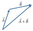
This motivates the following definition of vector addition, often called the tip-to-tail method. To add two vectors $\vec{A}$ and $\vec{B}$:
- place the tail of $\vec{B}$ at the tip of $\vec{A}$, then
- draw a new vector from the tail of $\vec{A}$ to the tip of $\vec{B}$.
This new vector is the sum of the two vectors, $\vec{A} + \vec{B}$.
When working with vectors in component form, we add or subtract the vectors by adding or subtracting their components separately. For example, if $\vec{A} = (A_x, A_y)$ and $\vec{B} = (B_x, B_y)$, then
\[\vec{A} + \vec{B} = (A_x + B_x, A_y + B_y),\]and
\[\vec{A} - \vec{B} = (A_x - B_x, A_y - B_y).\]Example: Adding and subtracting vectors
If $\vec{A} = \left(2\ \mathrm{m},\ 8\ \mathrm{m}\right)$ and $\vec{B} = \left(6\ \mathrm{m},\ 1\ \mathrm{m}\right)$, what are $\vec{A} + \vec{B}$ and $\vec{A} - \vec{B}$?
Solution
Using the previous formulas for vector addition and subtraction in terms of components, we have
\[\vec{A} + \vec{B} = (2\ \mathrm{m} + 6\ \mathrm{m},\ 8\ \mathrm{m} + 1\ \mathrm{m}) = (8\ \mathrm{m},\ 9\ \mathrm{m}),\] \[\vec{A} - \vec{B} = (2\ \mathrm{m} - 6\ \mathrm{m},\ 8\ \mathrm{m} - 1\ \mathrm{m}) = (-4\ \mathrm{m},\ 7\ \mathrm{m}).\]Changing velocity
The change in velocity $\Delta \vec{v}$ is the vector that points from the tip of $\vec{v}_1$ to the tip of $\vec{v}_2$. For example, consider the two velocity vectors from earlier:
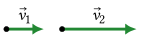
Placing the two vectors with their tails at the same point and drawing the vector from the tip of $\vec{v}_1$ to the tip of $\vec{v}_2$ gives us the change in velocity $\Delta \vec{v}$:

Since velocity is a vector, the velocity can change in both magnitude and direction. Here’s an example of a change in velocity that involves both a change in speed and a change in direction:
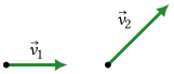
We can find $\Delta \vec{v}$ following the same procedure:

Average acceleration
The rate at which the velocity changes with time is called the acceleration $\vec{a}$.
Important: In physics, we use the word “acceleration” in a different way than you are used to from everyday language. In everyday language, to accelerate usually means to increase in speed. In physics, the acceleration is a vector that represents any change in the velocity vector. This could include any change in speed (both speeding up or slowing down), any change in direction, or both.
We define the average acceleration $\vec{a}_{\mathrm{av}}$ over a time interval $\Delta t$ as the change in velocity divided by the time interval:
\[\boxed{\vec{a}_{\mathrm{av}} = \frac{\Delta \vec{v}}{\Delta t} = \frac{\vec{v}_2 - \vec{v}_1}{\Delta t}.}\]Units of acceleration
The change in velocity $\Delta \vec{v}$ has units of $\mathrm{m/s}$, and the time interval $\Delta t$ has units of $\mathrm{s}$, so the units of average acceleration are $\mathrm{m/s^2}$, pronounced “meters per second squared.”
Some examples of acceleration magnitudes for reference:
- The rate at which objects accelerate due to gravity near the surface of the Earth is about $9.8\ \mathrm{m/s^2}$.
- A typical elevator has a maximum acceleration of about $1.0\ \mathrm{m/s^2}$.
- A Metro subway or light rail train has a maximum acceleration of about $1.5\ \mathrm{m/s^2}$.
- Roller coasters like Full Throttle at Six Flags Magic Mountain can briefly reach maximum accelerations of about $40\ \mathrm{m/s^2}$.
The direction of the acceleration vector
Since the average acceleration vector $\vec{a}_{\mathrm{av}}$ is defined as the change in velocity $\Delta \vec{v}$ divided by the time interval $\Delta t$, it points in the same direction as the change in velocity.
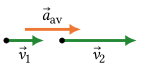
The direction of the average acceleration vector $\vec{a}_{\mathrm{av}}$ tells us the direction in which the velocity changes. On its own, this is not enough information to tell us whether the particle is speeding up or slowing down. We also need to know which way the velocity was pointing initially.
In both of the following examples, the average acceleration vector $\vec{a}_{\mathrm{av}}$ points to the right, but in the first example, the particle is speeding up, while in the second example, the particle is slowing down.
The particle is moving to the right and speeding up:
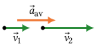
The particle is moving to the left and slowing down:
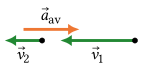
In general, when the velocity and acceleration vectors point in the same direction, the particle is speeding up, and when they point in opposite directions, the particle is slowing down.
Decomposing vectors
Finding the components of a vector given its magnitude and direction is called decomposing the vector. The direction of the vector is usually given as an angle $\theta$ measured from one of the coordinate axes. To start, let’s consider the case where the vector is in the first quadrant and $\theta$ is measured counterclockwise from the positive $x$-axis.
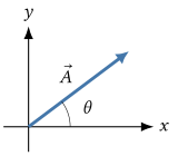
Start by drawing the vector $\vec{A}$ on the coordinate axes, with its tail at the origin. Then, draw a right triangle with $\vec{A}$ as the hypotenuse and the sides of the triangle parallel to the axes.
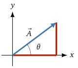
The side parallel to the $x$-axis is the $x$-component of $\vec{A}$, and the side parallel to the $y$-axis is the $y$-component of $\vec{A}$.
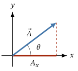
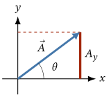
The magnitude of the vector is the length of the hypotenuse, and we can use the sine and cosine functions to relate the components to the magnitude.
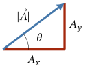
Recall that
\[\sin\theta = \frac{\text{opposite}}{\text{hypotenuse}} \quad \text{and} \quad \cos\theta = \frac{\text{adjacent}}{\text{hypotenuse}}.\]For the specific triangle in this example, the side opposite the angle $\theta$ is the $y$-component of $\vec{A}$, and the side adjacent to the angle $\theta$ is the $x$-component of $\vec{A}$. So we have
\[\sin\theta = \frac{A_y}{\lvert\vec{A}\rvert}, \quad\quad \cos\theta = \frac{A_x}{\lvert\vec{A}\rvert}.\]Rearranging these equations gives us formulas for the components of $\vec{A}$,
\[\begin{aligned} A_x &= \lvert\vec{A}\rvert \cos\theta, \\ A_y &= \lvert\vec{A}\rvert \sin\theta. \end{aligned}\]Note that this is just one example of how to decompose a vector! The formulas we got here for the components only work in the case when $\theta$ is the angle between the vector and the positive $x$-axis. If we started with a different angle, we would get different formulas for the components.
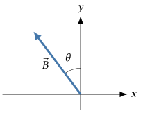
Check your understanding: Consider the following vector $\vec{B}$ in the second quadrant, where $\theta$ is measured counterclockwise from the positive $y$-axis. Repeat the same steps as before to find the components of $\vec{B}$ in terms of its magnitude and the angle $\theta$. (Pay attention to the signs of the components!)
Answer
For this vector and this angle, the components are
\[\begin{aligned} B_x &= -\lvert\vec{B}\rvert \sin\theta, \\ B_y &= \lvert\vec{B}\rvert \cos\theta. \end{aligned}\]In general, the process for decomposing a vector $\vec{A}$ is:
- Draw the vector on the coordinate axes, with its tail at the origin.
- Draw a right triangle with the vector as the hypotenuse, the sides of the triangle parallel to the coordinate axes, and the given angle $\theta$ interior to the triangle.
- Label the sides of the triangle as the absolute values of the components of the vector. The side opposite $\theta$ is $A \sin\theta$, and the side adjacent to $\theta$ is $A \cos\theta$.
- Determine the signs of the components based on which way the vector points along each axis (or equivalently, based on which quadrant the vector is in).
- Write the components of the vector in terms of its magnitude and the angle $\theta$ with the appropriate signs.
Calculating the magnitude and angle of a vector
We often want to find the magnitude of a vector given its components. For example, if we have a velocity vector $\vec{v} = (v_x, v_y)$, we might want to find the speed of the particle, which is the magnitude of the velocity vector.
We can use the same right triangle setup we used to find the components of a vector. The magnitude of the vector is the length of the hypotenuse, and we can use the Pythagorean theorem to find it in terms of the components. If we have a triangle with sides $a$ and $b$ and hypotenuse $c$, the Pythagorean theorem states that
\[c^2 = a^2 + b^2.\]Applying this to the triangle formed by a vector $\vec{A}$ and its components, we have
\[\lvert\vec{A}\rvert^2 = A_x^2 + A_y^2,\]so the magnitude of the vector is
\[\boxed{\lvert\vec{A}\rvert = \sqrt{A_x^2 + A_y^2}.}\]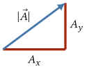
Angle of a vector
One way to specify the direction of a vector is to give the angle $\theta$ that the vector makes with one of the coordinate axes. Conventionally, we measure $\theta$ counterclockwise from the positive $x$-axis. To find the angle $\theta$ given the components of a vector, we can return to the expression for the sine and cosine of $\theta$ in terms of the components and magnitude of the vector:
\[\begin{aligned} A_x &= \lvert\vec{A}\rvert \cos\theta, \\ A_y &= \lvert\vec{A}\rvert \sin\theta. \end{aligned}\]Dividing the second equation by the first gives us
\[\tan\theta = \frac{A_y}{A_x}.\]Since $\tan\theta = A_y / A_x$, we can find the angle $\theta$ using the inverse tangent function:
\[\theta = \tan^{-1}\left(\frac{A_y}{A_x}\right).\]We have to be a little careful with this formula, because strictly speaking, it is only valid when the vector is in the first or fourth quadrants, so when the $x$-component of the vector is positive. To see why this is, let’s look at an example.
Example: Angle of a vector in the second quadrant
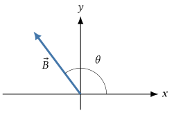
Find the angle $\theta$ that the vector $\vec{B} = (-3.0\ \mathrm{m},\ 4.0\ \mathrm{m})$ makes with the positive $x$-axis.
Solution
We want the angle $\theta$ that $\vec{B}$ makes with the positive $x$-axis, measured counterclockwise. The components of the vector are $B_x = -3.0\ \mathrm{m}$ and $B_y = 4.0\ \mathrm{m}$, so $\vec{B}$ lies in the second quadrant.
If we try to find $\theta$ using the inverse tangent function,
\[\theta = \tan^{-1}\left(\frac{B_y}{B_x}\right)\]we’ll find that we only get the correct answer when the vector is in the first or fourth quadrant, because the calculator’s $\tan^{-1}$ function always outputs an angle in the range $\left(-90^\circ,\ 90^\circ\right)$. If we just plug our numbers in, we get
\[\begin{aligned} \tan^{-1}\left(\frac{4.0\ \mathrm{m}}{-3.0\ \mathrm{m}}\right) &= \tan^{-1}(-1.333\ldots) \\ &\approx -53.13^\circ. \end{aligned}\]But $-53.13^\circ$ is an angle in the fourth quadrant, so this is the angle of the vector $\vec{C} = (3.0\ \mathrm{m},\ -4.0\ \mathrm{m})$, which is directly opposite our vector $\vec{B}$. That is not what we want.
Whenever the $x$-component is negative (second or third quadrant), we need to add $180^\circ$ to the calculator’s answer to rotate the angle into the correct quadrant. For our $\vec{B}$,
\[\begin{aligned} \theta &= -53.13^\circ + 180^\circ \\ &= 126.87^\circ \\ &\approx \boxed{127^\circ}. \end{aligned}\]Sanity check. A vector in the second quadrant should have an angle between $90^\circ$ and $180^\circ$ when measured counterclockwise from the positive $x$-axis. Our result $\theta \approx 127^\circ$ falls inside that range, so this answer is consistent.
Why the inverse tangent needs a quadrant check
There are two vectors that both have
\[\tan\theta = -\frac{4.0}{3.0}.\]One is our vector $\vec{B}$ in the second quadrant and the other is the vector $\vec{C} = (3.0\ \mathrm{m},\ -4.0\ \mathrm{m})$ in the fourth quadrant. The $\tan^{-1}$ function will only give us the angle for one of these vectors, so we have to use the signs of the components to determine which one is correct.
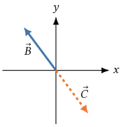
By convention, whenever there are two vectors that will give the same value for $\tan\theta$, the $\tan^{-1}$ function will give us the angle for the vector that has a positive $x$-component (in the first or fourth quadrants). In this example, the $\tan^{-1}$ function will give us the angle for the vector $\vec{C}$ in the fourth quadrant, so we have to add $180^\circ$ to get the angle for our vector $\vec{B}$ in the second quadrant.
In general, if we have a vector with a negative $x$-component, we need to add $180^\circ$ to the angle given by the $\tan^{-1}$ function to get the correct angle for the vector. If the vector has a positive $x$-component, then the angle given by the $\tan^{-1}$ function is already correct.
To summarize, the angle $\theta$ that a vector $\vec{A} = (A_x, A_y)$ makes with the positive $x$-axis is given by
\[\theta = \begin{cases} \tan^{-1}\left(A_y/A_x\right) & \text{if } A_x > 0, \\ \tan^{-1}\left(A_y/A_x\right) + 180^\circ & \text{if } A_x < 0. \end{cases}\]