Instantaneous velocity
We’ve seen how to calculate the average velocity over a time interval $\Delta t$. But what if we want to describe how a particle is moving at a specific instant in time? To do this, we need to define the instantaneous velocity of the particle at time $t$. To see how to define the instantaneous velocity, let’s take a moment to interpret the average velocity in terms of the particle’s position vs. time graphs.
Recall that the $x$-component of the average velocity over a time interval from $t_1$ to $t_2$ is given by
\[v_{\mathrm{av},x} = \frac{x(t_2) - x(t_1)}{t_2 - t_1}.\]This expression for the average velocity is exactly the slope of the line connecting the two points $(t_1, x(t_1))$ and $(t_2, x(t_2))$ on the position vs. time graph for the $x$-coordinate (what we call the secant line).
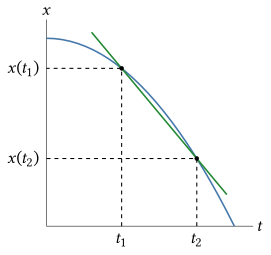
To calculate the instantaneous velocity, we would like to make the two times $t_1$ and $t_2$ the same. However, we can’t just set $t_1 = t_2$ in the formula for the average velocity, because then we would be dividing by zero. Instead, we need to take the limit of the average velocity as the time interval $\Delta t$ goes to zero. Intuitively, you can think of this as a process of shrinking the time interval down to be arbitrarily small but not exactly zero.
When we take the limit of the $x$-component of the average velocity, we get the slope of the tangent line to the $x$ position vs. time graph. This slope is the $x$-component of the instantaneous velocity at time $t$, and we write it as
\[\boxed{v_x(t) = \frac{dx}{dt}.}\]The slope of the tangent line is also called the derivative of $x$ with respect to $t$.
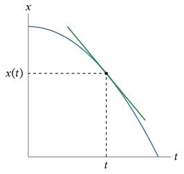
The slope $\frac{dx}{dt}$ of the tangent line at time $t$ is the $x$-component of the instantaneous velocity at time $t$.
I’ve written this equation for the $x$-component of the velocity, but it applies to the component of the velocity along any coordinate axis, whether we call it $x$, $y$, $\bigstar$, or whatever. For example, the $y$-component of the instantaneous velocity is given by
\[v_y(t) = \frac{dy}{dt},\]that is
\[v_y(t) = \text{slope of tangent line to the } y \text{ vs. } t \text{ graph at time } t.\]Check your understanding: The following figure shows a $y$ position vs. time graph for a ball tossed upwards. Sketch a $v_y$ vs. time graph for the ball.
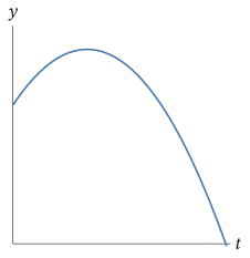
Answer
We can eyeball the $v_y$ vs. time from the given $y$ vs. time graph, since we know
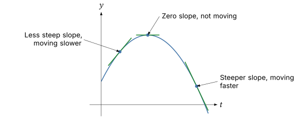
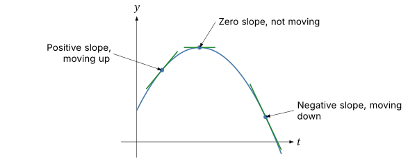
\[v_y(t) = \frac{dy}{dt} = \text{slope of the tangent line to the } y(t) \text{ curve at time } t.\]Picking a few representative points on the $y(t)$ curve and sketching the tangent lines, we see that the slope starts positive at $t = 0$, decreases to zero at the peak of the parabola, and then becomes negative and gets steeper as time increases.
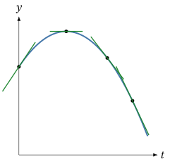
The $v_y(t)$ graph is therefore a straight line that starts positive (the ball is moving upward), passes through zero at the peak (where the ball is momentarily at rest in the vertical direction), and becomes increasingly negative as the ball falls back down.
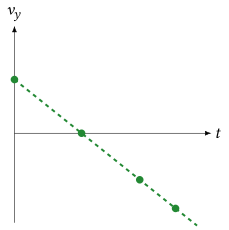
The magnitude of $v_y$ tells us the rate of motion along the corresponding coordinate axis.
The sign of $v_y$ indicates the direction of motion.
The velocity vector
Working in an $x$-$y$ coordinate system, we can write the instantaneous velocity vector in component form as
\[\begin{aligned} \vec{v} &= (v_x, v_y)\\ &= \left(\frac{dx}{dt}, \frac{dy}{dt}\right). \end{aligned}\]If we graph the path of the particle in the $x$-$y$ plane, then the velocity vector at any point on the path is tangent to the path at that point.
Example: Velocity vector from position graphs
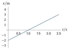
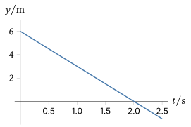
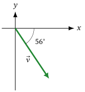
A particle moving in the $xy$ plane has $x$ and $y$ coordinates with the following position vs. time graphs. Find the magnitude and direction of the particle’s velocity vector.
Solution
The velocity components are the slopes of the $x(t)$ and $y(t)$ graphs. Both graphs are straight lines, so the slopes, and therefore both components of $\vec{v}$, are constant in time. We can read the slopes directly off the graphs.
From the $x(t)$ graph, the line starts at $(0\ \mathrm{s},\ -2\ \mathrm{m})$ and intersects the $t$-axis at $(1.0\ \mathrm{s},\ 0\ \mathrm{m})$, so
\[v_x = \frac{dx}{dt} = \frac{\Delta x}{\Delta t} = \frac{0\ \mathrm{m} - (-2\ \mathrm{m})}{1.0\ \mathrm{s} - 0\ \mathrm{s}} = \frac{2\ \mathrm{m}}{1.0\ \mathrm{s}} = 2\ \mathrm{m/s}.\]From the $y(t)$ graph, the line starts at $(0\ \mathrm{s},\ 6\ \mathrm{m})$ and intersects the $t$-axis at $(2\ \mathrm{s},\ 0\ \mathrm{m})$, so
\[v_y = \frac{dy}{dt} = \frac{\Delta y}{\Delta t} = \frac{0\ \mathrm{m} - 6\ \mathrm{m}}{2\ \mathrm{s} - 0\ \mathrm{s}} = -3\ \mathrm{m/s}.\]In component form,
\[\vec{v} = (v_x,\ v_y) = \boxed{(2\ \mathrm{m/s},\ -3\ \mathrm{m/s})}.\]Magnitude. Using the Pythagorean theorem,
\[\begin{aligned} |\vec{v}| &= \sqrt{v_x^2 + v_y^2} = \sqrt{(2\ \mathrm{m/s})^2 + (-3\ \mathrm{m/s})^2}\\ &= \sqrt{13\ \mathrm{m^2/s^2}} = \boxed{3.6\ \mathrm{m/s}}. \end{aligned}\]Direction. Because $v_x > 0$ and $v_y < 0$, the velocity vector is in the fourth quadrant. So we have
\[\theta = \tan^{-1}\!\left(\frac{v_y}{v_x}\right) = \tan^{-1}\!\left(\frac{-3\ \mathrm{m/s}}{2\ \mathrm{m/s}}\right) = \boxed{-56^\circ}\]that is, $56^\circ$ below the positive $x$-axis.
Uniform motion
Suppose we have a particle moving along a straight line, so we can use a single coordinate $x$ to describe the position of the particle. (Remember, we could call this coordinate $y$, $\bigstar$, or whatever we want, but I’ll stick with $x$ for now.)
Suppose the particle starts at $x(0) = x_0$. (We call the position at time $0$ the initial position of the particle.) How can we predict the particle’s $x$ coordinate at a later time $t$? In other words, how can we find a formula for $x(t)$?
If we know how the particle is moving at every instant in time—that is, if we know the $x$-component of the particle’s velocity at every time $t$—then we can find the position at any later time.
To see how this works, let’s consider the special case where the particle moves with a constant velocity. Motion with a constant velocity is called uniform motion.
We know that the velocity is the slope of the position vs. time graph, so the position vs. time graph for a particle in uniform motion is a straight line.
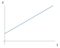
Because the velocity is constant, we can find the $x$-component of the velocity simply by finding the slope of the position vs. time graph. That is
\[v_x = \frac{\Delta x}{\Delta t}.\]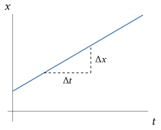
Note: This is only true when the velocity is constant. In general, the slope of the graph will not be constant, so to find the velocity we have to find the slope of the tangent line to the graph at a specific time $t$.
So in uniform motion the displacement over any time interval is just the velocity multiplied by the time interval:
\[\Delta x = v_x \Delta t.\]Starting from the initial position $x_0$ at time $t = 0$, we can find the position $x(t)$ at any later time $t$ by adding the displacement to the initial position:
\[\begin{aligned} \Delta x &= v_x \Delta t\\ \rightarrow x(t) - x_0 &= v_x (t - 0). \end{aligned}\]Rearranging for $x(t)$ gives us a formula for the position of a particle in uniform motion at any time $t$:
\[\boxed{x(t) = x_0 + v_x t}\]Notice that this is just the equation of a straight line with slope $v_x$ and $x$-intercept $x_0$, which is exactly what we expect from the graph of a particle in uniform motion.
Calculating displacement from velocity
How do we predict the position of a particle at a later time if the velocity is not constant? That is, suppose the velocity changes over time, but we know the velocity $v_x(t)$ at every time $t$. Given a particle’s initial position $x_0$, how can we find the position $x(t)$ at a later time $t$?
To see how to do this, let’s go back to the example of uniform motion, where we found that the displacement of a particle in uniform motion over a time interval $\Delta t$ is
\[\Delta x = v_x \Delta t.\]This formula for the displacement in uniform motion has a geometric interpretation: $\Delta x$ is the area of the rectangle with height $v_x$ and width $\Delta t$ under the velocity vs. time graph.
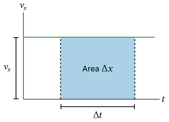
If the velocity is not constant, we can’t calculate the displacement using a single rectangle, but we can approximate the displacement by breaking the time interval into smaller subintervals and approximating the velocity as constant on each subinterval:
\[\Delta x \approx v_{1,x} \Delta t_1 + v_{2,x} \Delta t_2 + v_{3,x} \Delta t_3 + \ldots\]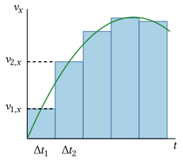
The smaller we make the subintervals, the better our approximation will be. In the limit where we make the subintervals infinitesimally small, the approximation becomes exact.
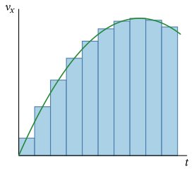
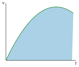
This means that if we want to calculate the displacement of a particle over a time interval, we can calculate the area between the velocity vs. time graph and the time axis over that time interval. Mathematically, this area is called the integral of the velocity function $v_x(t)$ with respect to time $t$ over the time interval $t_1$ to $t_2$. We write this as
\[\boxed{\Delta x = \int_{t_1}^{t_2} v_x(t)\,dt}\]Don’t worry if this notation is unfamiliar to you. This is just a short-hand way of saying
\[\boxed{\Delta x = \text{the area between the graph of } v_x(t) \text{ and the time axis from } t_1 \text{ to } t_2}\]Calculating position coordinates
Given the velocity function $v_x(t)$, we can calculate the area under the graph to find the displacement. In order to predict the position at a later time, we also need to know the initial position $x_0$ of the particle.
Taking the displacement from $t = 0$ to arbitrary time $t$, we can write
\[\Delta x = \int_0^t v_x(t')\,dt' \rightarrow x(t) - x_0 = \int_0^t v_x(t')\,dt'\]Rearranging for $x(t)$ gives us a formula for the position of a particle at any time $t$ given its initial position and its velocity function:
\[x(t) = x_0 + \int_0^t v_x(t')\,dt'\]Example: Position from a piecewise velocity graph
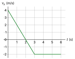
The plot below shows a velocity vs. time graph for an object that starts at $x = -2.0\ \mathrm{m}$ at $t = 0$. Find the position of the object at $t = 5.0\ \mathrm{s}$.
Solution
The graph has two distinct segments:
- From $t = 0$ to $t = 3\ \mathrm{s}$, $v_x$ decreases steadily along a straight line from $4\ \mathrm{m/s}$ down to $-2\ \mathrm{m/s}$.
- From $t = 3\ \mathrm{s}$ to $t = 6\ \mathrm{s}$, $v_x$ is constant at $-2.0\ \mathrm{m/s}$.
The velocity crosses zero at $t = 2.0\ \mathrm{s}$ (where the sloped line intersects the time axis). This is a turning point where the object momentarily stops and changes direction.
To find the position at $t = 5.0\ \mathrm{s}$, we use the area under the velocity curve to find the displacement $\Delta x$ from $t = 0$ to $t = 5.0\ \mathrm{s}$. We can break this area up into three pieces: the triangle from $t = 0$ to $t = 2.0\ \mathrm{s}$, the triangle from $t = 2.0\ \mathrm{s}$ to $t = 3.0\ \mathrm{s}$, and the rectangle from $t = 3.0\ \mathrm{s}$ to $t = 5.0\ \mathrm{s}$. Label the areas of these three pieces $\Delta x_1$, $\Delta x_2$, and $\Delta x_3$ respectively.
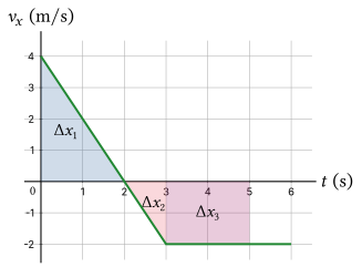
Using the formulas for the areas of triangles and rectangles, we have
\[\begin{aligned} \Delta x_1 &= \tfrac{1}{2} (2.0\ \mathrm{s})(4.0\ \mathrm{m/s}) = 4.0\ \mathrm{m},\\ \Delta x_2 &= \tfrac{1}{2} (1.0\ \mathrm{s})(-2.0\ \mathrm{m/s}) = -1.0\ \mathrm{m},\\ \Delta x_3 &= (2.0\ \mathrm{s})(-2.0\ \mathrm{m/s}) = -4.0\ \mathrm{m}. \end{aligned}\]Note that $\Delta x_2$ and $\Delta x_3$ are negative because the object is moving in the $-x$ direction over those intervals (the velocity is below the axis). Adding these up gives the total displacement from $t = 0$ to $t = 5.0\ \mathrm{s}$:
\[\Delta x = \Delta x_1 + \Delta x_2 + \Delta x_3 = 4.0\ \mathrm{m} - 1.0\ \mathrm{m} - 4.0\ \mathrm{m} = -1.0\ \mathrm{m}.\]Finally, the position at $t = 5.0\ \mathrm{s}$ is the initial position plus the displacement:
\[x(5.0\ \mathrm{s}) = x_0 + \Delta x = -2.0\ \mathrm{m} - 1.0\ \mathrm{m} = \boxed{-3.0\ \mathrm{m}.}\]