Review: solving a kinematics problem
Before we introduce acceleration, let’s review the ideas of velocity and displacement by working through a kinematics problem, practicing the general problem-solving steps from the previous chapter.
Example: Two dogs meeting
Two dogs, Max and Luna, run toward each other. Luna runs east at $5.0\ \mathrm{m/s}$. Max starts $50\ \mathrm{m}$ east of Luna and runs west at $4.0\ \mathrm{m/s}$.
a. How long does it take the dogs to meet?
b. Where are they when they meet?
c. Sketch position vs. time graphs for the two dogs, and indicate the time and location the dogs meet on your graph.
Solution
We can use this problem to walk through the eight-step problem-solving process.
Step 1: Draw a picture. Sketch a horizontal $x$-axis pointing east. Luna is at the origin with a velocity arrow of magnitude $5.0\ \mathrm{m/s}$ pointing east (to the right), and Max is at $x = 50\ \mathrm{m}$ with a velocity arrow of magnitude $4.0\ \mathrm{m/s}$ pointing west (to the left).

Step 2: Choose a coordinate system. Take the $+x$ axis pointing east, with $x = 0$ at Luna’s starting position. With this choice, Luna moves in the $+x$ direction and Max moves in the $-x$ direction.
Step 3: Define symbols and list what you know. Let $d = 50\ \mathrm{m}$ be the initial distance between the dogs. Let $v_L = 5.0\ \mathrm{m/s}$ be Luna’s speed and $v_M = 4.0\ \mathrm{m/s}$ be Max’s speed.
Step 4: Identify the goal. We want the time $t_1$ when the dogs meet, and the position $x_1$ where they meet.
Step 5: Physical conditions. The dogs meet when they are at the same location, which means that their position functions are equal at time $t_1$: $x_L(t_1) = x_M(t_1)$.
Step 6: Write down relevant equations. Both dogs move in uniform motion, so their position functions are of the form
\[x(t) = x_0 + v_x t,\]where $x_0$ is the initial position and $v_x$ is the $x$-component of the velocity. For Luna, $x_{L,0} = 0$ and $v_{L,x} = v_L$, so
\[x_L(t) = v_L t.\]For Max, $x_{M,0} = d$ and $v_{M,x} = -v_M$ (negative because Max moves west), so
\[x_M(t) = d - v_M t.\]Step 7: Solve. Setting the two position functions equal and solving for $t_1$,
\[\begin{aligned} v_L t_1 &= d - v_M t_1\\ \rightarrow v_L t_1 + v_M t_1 &= d\\ \rightarrow (v_L + v_M)\, t_1 &= d\\ \rightarrow t_1 &= \frac{d}{v_L + v_M} \end{aligned}\]Plugging in the given numbers, we get
\[\begin{aligned} t_1 &= \frac{50\ \mathrm{m}}{5.0\ \mathrm{m/s} + 4.0\ \mathrm{m/s}}\\ &= \boxed{5.6\ \mathrm{s}.} \end{aligned}\]To find the meeting position $x_1$, we can plug $t_1$ into either position function (since the dogs are at the same position at that time). Using Luna’s position,
\[\begin{aligned} x_1 &= v_L t_1\\ &= (5.0\ \mathrm{m/s})(5.6\ \mathrm{s})\\ &= \boxed{28\ \mathrm{m}.} \end{aligned}\]Step 8: Check our answer.
- Units: The time is in seconds and the position is in meters, which are the correct units for these quantities. ✓
- Reasonable numbers: The dogs start 50 meters apart and run toward each other at (what we can assume are) realistic speeds for dogs, so it seems reasonable that they would meet after a few seconds. The meeting point is close to halfway between the dogs’ starting positions, and slightly closer to Max’s starting position, which makes sense since Luna is faster than Max. So the answers seem physically reasonable. ✓
- Changing parameters: If the dogs started farther apart, we expect the time it would take them to reach each other to increase, and we see that $t_1$ is directly proportional to $d$. If the dogs ran faster, we expect the meeting time to decrease, and $t_1$ is inversely proportional to the sum of the speeds. So the answers have the correct dependence on the parameters. ✓
Part (c): position vs. time graphs. Both position functions are straight lines. Luna’s line starts at the origin with slope $+5.0\ \mathrm{m/s}$, and Max’s line starts at $50\ \mathrm{m}$ with slope $-4.0\ \mathrm{m/s}$. The two lines cross at the meeting point, $t_1 = 5.6\ \mathrm{s}$ and $x_1 = 28\ \mathrm{m}$, which you can mark with a dot and dashed lines connecting it to the axes.
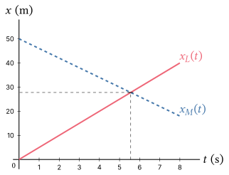
This example demonstrates a common pattern in kinematics problems: solving for a time when some condition holds, and then plugging that time into a function of time to find other information. In this specific problem, we first solve for the time $t_1$ when the dogs are at the same position, so when $x_L(t) = x_M(t)$. Then we plug that time into the position equation $x_L(t)$ or $x_M(t)$ to find the position where they meet.
Instantaneous acceleration
Just like we defined the instantaneous velocity as the limit of the average velocity, we can define the instantaneous acceleration as the limit of the average acceleration. Recall that the average acceleration is defined as the change in velocity divided by the change in time:
\[\vec{a}_{\mathrm{av}} = \frac{\Delta \vec{v}}{\Delta t}\]so, for example, the $x$-component of the average acceleration is
\[a_{\mathrm{av},x} = \frac{\Delta v_x}{\Delta t}.\]If we take the limit as $\Delta t \to 0$, we get the $x$-component of the instantaneous acceleration:
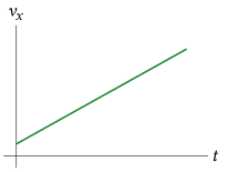
\[\boxed{a_x = \frac{dv_x}{dt}}\]Just as the instantaneous velocity is the slope of the position vs. time graph, the instantaneous acceleration is the slope of the velocity vs. time graph. A positive $a_x$ means $v_x$ is increasing:
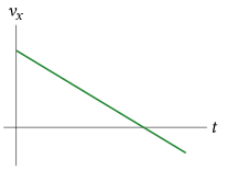
A negative $a_x$ means $v_x$ is decreasing:
Acceleration and position
Since the velocity is the derivative of the position,
\[v_x = \frac{dx}{dt},\]the acceleration is the second derivative of the position:
\[\begin{aligned} a_x &= \frac{d}{dt}\left(\frac{dx}{dt}\right)\\ &= \frac{d^2 x}{dt^2} \end{aligned}\]The second derivative tells us the curvature or concavity of the position vs. time graph:
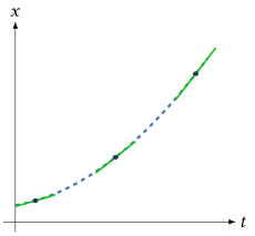
- If $a_x > 0$, the $x$ vs. $t$ graph is concave up.
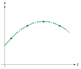
- If $a_x < 0$, the $x$ vs. $t$ graph is concave down.
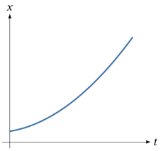
A concave up position vs. time graph ($a_x > 0$) has a slope that increases with time (increasing velocity):
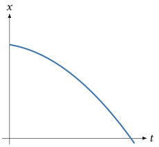
A concave down position vs. time graph ($a_x < 0$) has a slope that decreases with time (decreasing velocity):
Constant acceleration motion
Velocity in constant acceleration motion
Just like the displacement is the area under the $v_x(t)$ graph, the change in velocity is the area under the $a_x(t)$ graph. For constant acceleration, that area is a rectangle:
\[\Delta v_x = a_x \Delta t.\]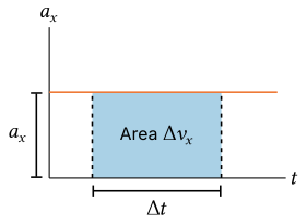
If a particle moving with constant acceleration $a_x$ starts with initial velocity $v_x(0) = v_{0x}$, then the velocity at time $t$ is
\[\boxed{v_x(t) = v_{0x} + a_x t.}\]This is our constant acceleration velocity equation. Once we have the velocity equation, we can find the position from the area under the velocity vs. time graph.
Position in constant acceleration motion
For constant acceleration, the area under the $v_x(t)$ graph is a trapezoid. Decomposing it into a rectangle and triangle gives
\[\Delta x = v_{0x} t + \tfrac{1}{2} a_x t^2.\]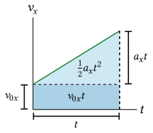
For a particle starting at initial position $x(0) = x_0$, the position at time $t$ is
\[\boxed{x(t) = x_0 + v_{0x} t + \frac{1}{2} a_x t^2.}\]This is our constant acceleration position equation.
What we call the coordinates doesn’t matter
Don’t assume that because I am writing formulas for the $x$-component of position, velocity, and acceleration, that the motion has to be along the $x$-axis or in the horizontal direction! $x$ is just a placeholder for whatever coordinate we choose to describe the motion.
These same formulas apply to constant acceleration motion along any axis or in any direction. For example, along a $y$ coordinate axis, the formulas would be
\[\begin{aligned} y(t) &= y_0 + v_{0y} t + \frac{1}{2} a_y t^2,\\ v_y(t) &= v_{0y} + a_y t. \end{aligned}\]Graphing constant acceleration motion
Since the position of an object in constant acceleration motion is a quadratic function of time, the position vs. time graph is a parabola. For $a_x > 0$, we get a concave up parabola:
For $a_x < 0$, we get a concave down parabola:
Example: Sketching $x(t)$ from a piecewise velocity graph
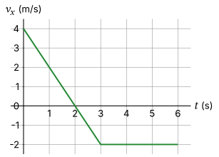
The plot below shows a velocity vs. time graph for an object that starts at $x = 0$ at $t = 0$. Sketch a position vs. time graph for the motion of the object from $t = 0$ to $t = 6$ seconds.
Solution
To sketch $x(t)$, we need the shape of the curve on each segment and the key times where the shape changes. The velocity graph has two segments:
-
From $t = 0$ to $t = 3\ \mathrm{s}$, $v_x$ is a straight line decreasing from $4\ \mathrm{m/s}$ to $-2\ \mathrm{m/s}$. The slope is constant, so this is constant-acceleration motion with
\[a_x = \frac{-2\ \mathrm{m/s} - 4\ \mathrm{m/s}}{3\ \mathrm{s} - 0\ \mathrm{s}} = -2.0\ \mathrm{m/s^2}.\]Because $a_x$ is constant and negative, $x(t)$ is a concave-down parabola on this segment.
-
From $t = 3\ \mathrm{s}$ to $t = 6\ \mathrm{s}$, $v_x$ is constant at $-2.0\ \mathrm{m/s}$, so $a_x = 0$ and $x(t)$ is a straight line with slope $-2.0\ \mathrm{m/s}$.
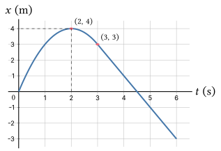
Key positions.
- Turning point at $t = 2\ \mathrm{s}$: the velocity crosses zero here, so the parabola reaches its peak.
- Crossover at $t = 3\ \mathrm{s}$: where the parabola joins the straight line.
Drawing the concave-down parabola from $(0,\ 0)$ up to the turning point and down to the crossover, then the straight line of slope $-2.0\ \mathrm{m/s}$, we get the following sketch for $x(t)$.
Turning points in constant acceleration motion
A particle with velocity and acceleration in opposite directions will eventually stop and change direction at a turning point. At a turning point, the velocity is instantaneously zero.
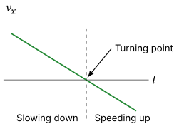
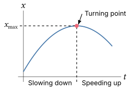
One example of a turning point is at the peak of the motion of a ball thrown straight up in the air. At the peak, the velocity is zero, and the ball changes direction from moving upward to moving downward.
The “$v^2$ equation”
There is a third equation for constant acceleration motion that is often useful, especially when we don’t know the time. We can derive it by solving for $t$ in the velocity equation and plugging that into the position equation:
\[\begin{aligned} \Delta t &= \frac{v_{f,x} - v_{i,x}}{a_x},\\ x_f &= x_i + v_{i,x} \Delta t + \frac{1}{2} a_x (\Delta t)^2. \end{aligned}\]After some algebra, we get
\[\boxed{v_{f,x}^2 = v_{i,x}^2 + 2 a_x \Delta x.}\]where $\Delta x = x_f - x_i$ is the displacement. There isn’t a standard name for this equation, so I usually just refer to it as the “$v$ squared equation.”
Example: Toy car with constant leftward acceleration
A toy car rolls on a horizontal surface and is initially moving right at $12.0\ \mathrm{m/s}$. The car has a constant acceleration directed to the left with magnitude $3.00\ \mathrm{m/s^2}$.
a. When does the car return to its starting point (after $t = 0$)?
b. What is the maximum distance to the right of its starting point that the car reaches?
Solution
Take $+x$ to the right, with the origin at the car’s starting point. We are given the initial position, velocity, and acceleration components,
\[x_0 = 0, \qquad v_{0x} = +12.0\ \mathrm{m/s}, \qquad a_x = -3.00\ \mathrm{m/s^2}.\]The acceleration is negative because it points in the $-x$ direction. Since the acceleration is constant, we can use the constant-acceleration kinematic equations:
\[\begin{aligned} v_x(t) &= v_{0x} + a_x t,\\ x(t) &= x_0 + v_{0x}\,t + \tfrac{1}{2} a_x t^{2}. \end{aligned}\](a) The car is back at its starting point when $x(t) = 0$. Setting the position function to zero,
\[v_{0x}\,t + \tfrac{1}{2} a_x t^{2} = 0.\]Since the problem asks for the time after $t = 0$, we can divide the equation by $t$ to get
\[v_{0x} + \tfrac{1}{2} a_x t = 0,\]and rearranging gives the return time
\[t_{\mathrm{ret}} = -\frac{2 v_{0x}}{a_x} = -\frac{2\,(12.0\ \mathrm{m/s})}{-3.00\ \mathrm{m/s^2}} = \boxed{8.00\ \mathrm{s}.}\](b) The car reaches its maximum position at the turning point, where its velocity is instantaneously zero. From the velocity equation,
\[\begin{aligned} 0 &= v_{0x} + a_x t_{\mathrm{max}}\\ \rightarrow t_{\mathrm{max}} &= -\frac{v_{0x}}{a_x} = -\frac{12.0\ \mathrm{m/s}}{-3.00\ \mathrm{m/s^2}} = 4.00\ \mathrm{s}. \end{aligned}\]Plugging this back into the position function,
\[\begin{aligned} x_{\max} &= x(t_{\mathrm{max}}) = v_{0x}\,t_{\mathrm{max}} + \tfrac{1}{2} a_x (t_{\mathrm{max}})^{2}\\ &= (12.0\ \mathrm{m/s})(4.00\ \mathrm{s}) - \tfrac{1}{2}(3.00\ \mathrm{m/s^2})(4.00\ \mathrm{s})^{2}\\ &= \boxed{24.0\ \mathrm{m}.} \end{aligned}\]Alternatively, we can skip computing $t_{\mathrm{max}}$ altogether by using the $v^2$ equation with final velocity $v_x = 0$ at the turning point:
\[\begin{aligned} 0 &= v_{0x}^{2} + 2\,a_x\,\Delta x_{\max}\\ \rightarrow \Delta x_{\max} &= -\frac{v_{0x}^{2}}{2\,a_x} = -\frac{(12.0\ \mathrm{m/s})^{2}}{2\,(-3.00\ \mathrm{m/s^2})} = 24.0\ \mathrm{m}.\ \checkmark \end{aligned}\]Both methods agree. Notice also that $t_{\mathrm{ret}} = 2\,t_{\mathrm{max}}$: by the symmetry of constant-acceleration motion, the trip out to the turning point and back takes equal times.
Symmetry of constant acceleration motion
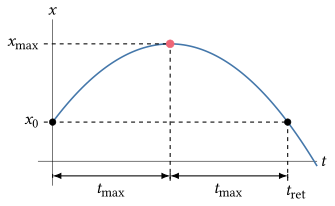
In the previous example, we found that the time to return to the starting point is $t_{\mathrm{ret}} = 8.00\ \mathrm{s}$. The time to reach the maximum distance is exactly half of that, $t_{\mathrm{max}} = 4.00\ \mathrm{s} = t_{\mathrm{ret}}/2$.
This is not a coincidence, but a consequence of the symmetry of constant acceleration motion. The motion from $t = 0$ to $t = t_{\mathrm{max}}$ is a “mirror image” of the motion from $t = t_{\mathrm{max}}$ to $t = t_{\mathrm{ret}}$.
In particular, when an object moves in constant acceleration motion with the acceleration opposite the initial velocity, the time to reach the turning point ($t_{\mathrm{max}}$) is always half of the time to return to the starting point ($t_{\mathrm{ret}}$):
\[\boxed{t_{\mathrm{max}} = \frac{t_{\mathrm{ret}}}{2}.}\]